An Introduction to the Theory of Cellular Automata

Published: October 14, 2024

1. Basic of Cellular Automata

1.1 What are Cellular Automata

You might have heard of Conway’s Game of Life, though calling it a “game” is somewhat misleading – it is more accurately described as a simulation. The Game of Life models the process of life on a grid of arbitrary size, where each square, or “tile,” can either be colored (alive) or uncolored (dead). The initial pattern of living cells can be set manually or randomized. From there, the simulation follows a set of simple rules that determine whether each cell will live, die, or remain unchanged in the next generation. The process repeats step by step until the user decides to stop it.

It’s called the Game of Life because it mimics biological life, with colored tiles representing living cells and non-colored ones representing dead cells. The rules simulate conditions for survival, birth, or death of these cells.

For more detail, I highly recommend checking out this aweasome Numberphile video with the game’s creator.

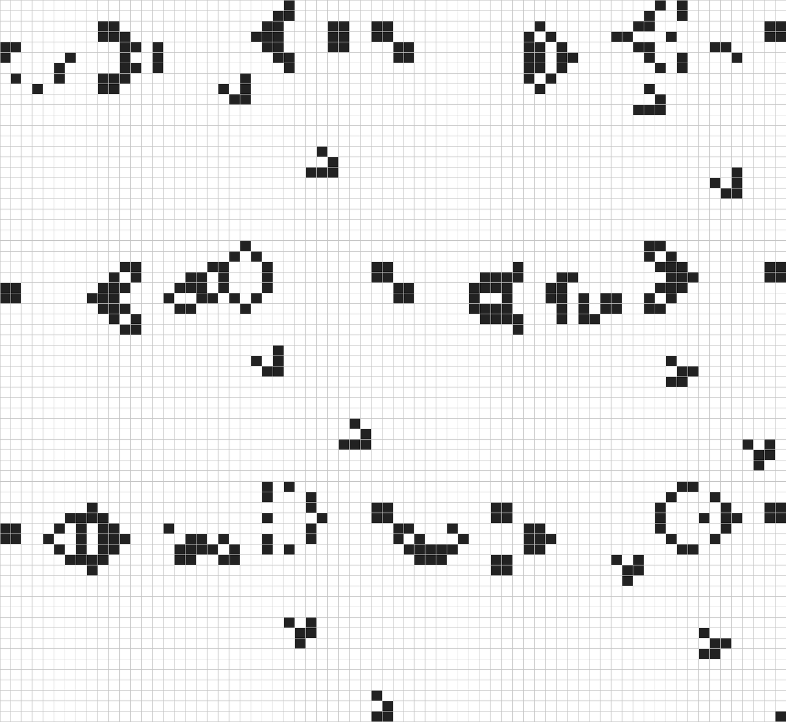
While Conway’s Game of Life is interesting, as true students of theoretical computer science, the first questions we should asks are: How can we formally describe this process? How can we generalize Conway’s Game of Life? These are the topics I’d like to explore in this article.

In the broadest terms, cellular automata(CA) are a computational model similar to finite state machines and Turing machines. In cellular automata, we have a grid of cells, each of which can exist in a finite number of states. At each step, all cells change their state simultaneously according to a predefined set of rules. Like finite state machines and Turing machines, cellular automata can be used to perform certain computations.

To fully understand the concepts presented in this article, it is required to have a basic understanding of the following prerequisites:

• Fundamentals of formal computer science language (e.g., Cartesian product)
• Basics of computability theory (e.g., Chomsky hierarchy)
• Big O notation

I will be using some technical jargon throughout this article, so knowing these topics is rather important.

1.2 Why use Cellular Automata?

Why should we care about the cellular automata computational model? Theoretical computer science often resembles mathematics in that we explore topics that may not have immediate practical applications, yet we explore them nonetheless. Why? It’s the same as to ask why a painter paints, a sculptor sculpts, and a photographer captures images: to try to capture the beauty in front of them, trying to grasp the Platonic ideal of beauty.

While that is a noble pursuit, cellular automata offer more than just that. In traditional computational paradigms, instructions are executed sequentially, one after another. In contrast, cellular automata allow all cells to update simultaneously, leading to significant speedups in solving certain problems. For instance, the fastest general comparison sorting algorithm with a Turing machine operates in \(O(n \log n)\), whereas with cellular automata, we can achieve sorting in \(O(n)\) under specific conditions.

Furthermore, cellular automata are often useful in simulations, particularly in scenarios involving gases or fluids. For instance, they have been utilized to investigate ways to improve the taste of coffee by simulating the brewing process. Another example of cellular automata being used for simulation purposes is the game Noita, where the entire environment is fully destructible, thanks to its physics engine, which heavily utilizes cellular automata.

1.3 Basic Definition

1.3.1 Definition – The Space \(R\) of a cellular automata, is defined as \(R = \mathbb{Z}_1 \times ... \times \mathbb{Z}_1\) where we call \(d\) the dimensionality of the Space. We can identify a given cell through the usage of coordiantes \(i = (i_1, ..., i_d)\). We furthmore have a set of finite states \(Q\). A global configuration is defined as \(c : R \to Q\) i.e. each cell gets assigned one state.

1.3.2 Example – Our space is \(R = \mathbb{Z}_1 \times \mathbb{Z}_2\), we have four states \(Q = \{\text{Brown, Black, Beige, Purple}\}\).

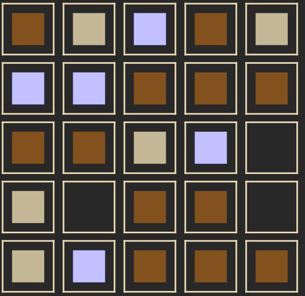
In the most simple case our cellular automata works deterministic, though it can also work asynchronous or probabilistic.

1.3.3 Definition – A neighborhood, is a finite set \(N = \{n_1, ..., n_k\} \subset \mathbb{Z}^d\). Where \(\mathbb{Z}^d\) is not the Space \(R\). The neighborhood of a cell \(i\) is \(n(i) := n + i\), this means we can get the \(j\)-th neighbor from the cell \(i\) like this \(i + n_j\). We call the mapping \(l : N \to Q\) a local configuration i.e. this describes a possible distribution of states in a neighborhood.

1.3.4 Definition – The d-dimensional Moore-Neighborhood with radius \(r\) we call \(M_r^d\) and is defined as \(M_r^d := \{(i_1,...,i_d) | \max_j |i| \leq r \}\). The d-dimensional Non-Neuman-Neighborhood with radius \(r\) ist \(N_r^d = \{(i_1,...,i_d) | \sum |i_j| \leq r\}\).

1.3.5 Definition – How a deterministic cellular automata works, is defined through the local transfer function \(\sigma: Q^N \to Q\) i.e. this mapping assigns a cell based, on the state of its neighbors, a new state.

1.3.6 Definition – If we have a global configuration \(c\), then we call the mapping \(c_{i + N} : N \to Q, n \mapsto c_{i+n}\) the local configuration at i in c i.e. \(c_{i + N}\) gives you for every neighbor for the cell i in the configuration c, its state \(c_{i + n}\). (Notice \(n\) is not \(N\)).

1.3.7 Definition – The global transfer function is defined as \(\Delta : Q^R \to Q^R \) with \(\Delta(c)_i = \sigma(c_{i + N})\) i.e. this function assign each cell its new state.

This CA is now strictly synchronous, because in each step all cell switch their state at the same time, like defined through the global transfer function.

1.3.8 Example – Now that we have introduced the basic concepts of the formal language of cellular automata (CA), we can return to Conway’s Game of Life and examine how it is defined.

In Conway’s Game of Life, we have the following parameters for the cellular automaton:

• Space: \( R = \mathbb{Z}^2 \) (the two-dimensional grid of cells)
• Neighborhood: \( N = M_{1}^2 \) (the adjacent cells)
• States: \( Q = \{0, 1\} \) (where 0 represents a dead cell and 1 represents a live cell)

The local transition function is defined as follows:

$$ \sigma(l) = \begin{cases} 1, & \text{if } l(0,0) = 0 \land s(l) = 3 \\ 1, & \text{if } l(0,0) = 1 \land 2 \leq s(l) \leq 3 \\ 0, & \text{otherwise} \end{cases} $$

Here, the helper function \( s(l) = \sum_{n \in N, n \neq (0,0)} l(n) \) counts the number of alive neighbors around the cell at \( (0, 0) \).

• The first case states that if a cell is dead (i.e., \( l(0,0) = 0 \)) and has exactly 3 alive neighbors, it becomes alive again.
• The second case indicates that if a cell is alive (i.e., \( l(0,0) = 1 \)) and has between 2 and 3 alive neighbors, it remains alive.
• The third case specifies that if an alive cell has more than 3 alive neighbors, it dies due to overcrowding.

For more information about Conway’s Game of Life, including specific patterns that emerge, check out the following blog post.

2. Computability Theory of Cellular Automata

2.1 Lemma – There exists a synchronous, deterministic, two-dimensional cellular automaton with an \(M_1^2\) neighborhood and four states, capable of simulating any finite state machine (with an arbitrarily sized state set and arbitrary transition function).

How can we prove this?
First, we introduce a new cellular automaton called Wireworld.
Wireworld has the state set \(Q = \{\text{Brown, Black, Beige, Purple}\}\), and we use the \(M_1^2\) neighborhood.
The local transition function is shown below, where a cross indicates that the state is irrelevant, and a question mark indicates that the states matter when moving to the next step.

The Beige state represents copper in wires, and the combination of Purple and White represents a signal flowing through the wire.
We can now use Wireworld to simulate various electrical devices by smartly choosing the initial configuration of space \(R\) and applying the transition function repeatedly. Below, you can see the simulation of a wire with a signal flowing through it.

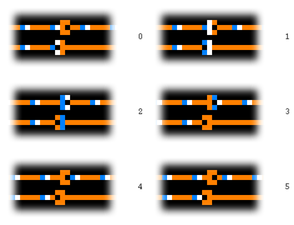
It is also possible to simulate a diode, where a signal can flow in one direction but not in the other. As shown, the signal in the top wire passes through the diode, while in the second wire it does not. Why? If you think back to the local transition function, a cell only turns blue when one or two neighboring cells are blue. In the top wire, this condition is met. In the bottom wire, at the end of the diode, we have three blue cells, so the signal doesn’t propagate further.

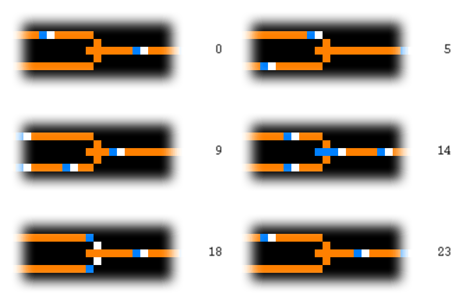
A diode is interesting, but even more useful is an OR-gate. The construction is simple: we join two wires together, but we add one more copper cell at the left side where the wires meet. This prevents the signal from propagating back to the other wire when only one signal reaches the OR-gate.

Similarly, we can use initial configurations to simulate an inverter, exclusive-OR, AND, and a clock generator, which can generate signals. Using these elements, we can build a ROM and other components necessary for a computer. You can find more information about this on the Quinapalus website, where the gifs of the simulations shown above are also from.

Back to the proof – Now that we have introduced Wireworld and the various components it can simulate, we can return to the proof. Remember, we wanted to prove that we can use a CA to simulate a finite state machine.
We define a <1> signal as having a 1 (blue cell) followed by nothing for 22 steps. A <0> signal is defined as having nothing for 23 steps. With this, we can fit all previously introduced electrical elements into a 24x24 cell grid. When we have a signal at the beginning of one of these elements, we can be sure that 48 steps later, it will reach the output, thus allowing us to synchronize the components. This allows us to simulate a finite state machine using our 24x24 cell grid logic gates.

2.2 Lemma – For every Turing machine \(T=(Q_T, B_T, \delta_T)\), there exists a synchronous cellular automaton \(C = (Q_C, \delta_C, H_1^1)\) that can simulate the Turing machine step-by-step without time loss.

In a Turing machine (TM), we have a tape representing the current storage. We can simulate this using a one-dimensional cellular automaton, where the tape’s contents are stored in the cells. Additionally, we mark the cell in the CA corresponding to the position of the Turing machine’s head, while the other cells in the CA contain an underscore “_” to indicate that the head is not on those cells.

This means we represent a TM configuration \(c_T = (s, b, p)\) through a CA configuration as follows, where \(Q_C\) is the state set of the CA defined as \(C_C = (Q_T \cup \{\_\}) \times B_T\):

Now we need a transition function that translates each step of the Turing machine into a step in the CA. The following are some of the most important steps:

For example, in the first line of the image above, if the current cell and its left and right neighbors are not active (i.e., the TM head is not on them), then nothing changes in our cell.
In the second line, if our current cell is not active, but the cell to its left is, we activate the current cell if the Turing machine’s transition function dictates a move to the right from the active cell.

As an example, the following shows the configuration of a Turing machine for a given initial state:

And here is how the CA that simulates the TM would look:

The crossed lines indicate that each cell in the CA can have two possible values. This is achieved by defining the set of states \(Q_C\) as the Cartesian product of \(Q_T\) (the states of the Turing machine) with \(B_T\) (the states of the Turing machine’s transition function).

3. Finite Patterns and Configurations

Definition 3.1 – A subset \(P \subset Q\) is called passive if, for all \(l: N \to Q\) and \(n \in N\) where \(l(n) \in P\), it holds that \(\delta(l) = \delta(0)\).
A state \(q \in Q\) is called a resting state if \(\{q\}\) is passive, meaning that \(\delta(q, q, \dots, q) = q\).
A state \(t \in Q\) is called dead if for all \(l: N \to Q\) with \(l(0) = t\), it holds that \(\delta(l) = t\).

In simpler terms, a subset is passive if, for all cells, it is true that when all their neighbors are in a state from the passive set, the cells do not change state in the next step.
A state is dead if cells in this state never change, regardless of the state of their neighborhood.

Example 3.2 – In Wireworld, \(\{\text{White, Beige}\}\) form a passive set, and \(\{\text{White}\}\) is a dead state.

Definition 3.3 – Let \(C\) be a d-dimensional cellular automaton with space \(R\) and a resting state \(q\). A pattern is a mapping \(m: T \to Q \backslash \{q\}\), where \(T \subset Q\) and is called the carrier.
Furthermore, we define the associated pattern configuration \(c_m: R \to Q\) by:

\[ c_m(i) = \begin{cases} m(i), \ \text{if } i \in T \\ q, \quad \ \ \text{otherwise} \end{cases} \]

A pattern \(m\) exists in a configuration \(c\) at position \(j\) if \(\forall i \in T: c(j + i) = m(i)\).

This means a pattern is a mapping from a portion of space \(R\) to certain states in the state set \(Q\). The pattern is translation-invariant, meaning it can appear at any coordinate in space, e.g., at space \(j\).
A pattern configuration is a configuration where the pattern is filled with resting states.

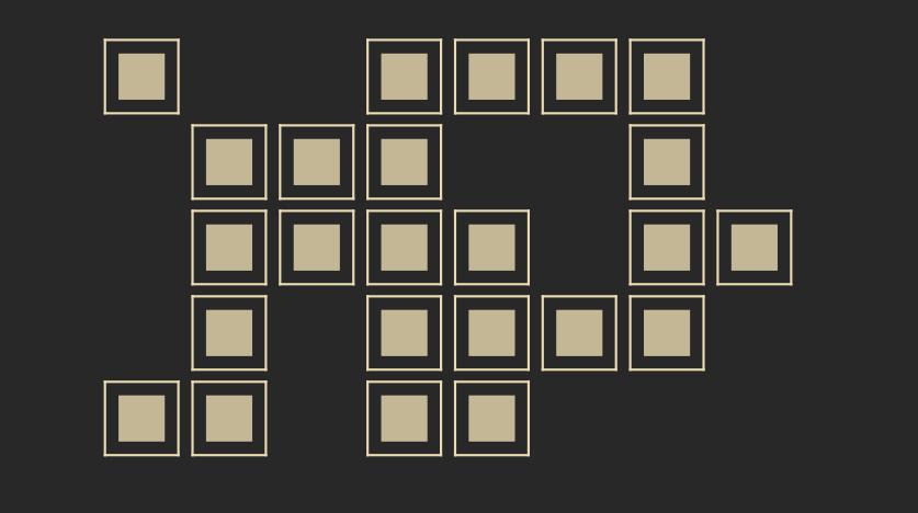
Example 3.4 – Often, 1-dimensional patterns are words. A simple 2-dimensional pattern could be a rectangle \(m: \mathbb{N}_n \times \mathbb{N}_m \to Q\), but patterns can also be irregular:

Definition 3.5 – The input of a pattern \(m\) into a corresponding cellular automaton happens through choosing the pattern configuration as the start configuration.
A configuration is in its end configuration when \(\Delta(c) = c\); that is, when we apply the transition function and no further changes occur.

Definition 3.6 – A configuration \(c: R \to Q\) has the carrier \(T(c) = \{i \mid c_i \neq q\}\). A configuration is finite if its carrier is finite. This means we disregard passive states when considering the carrier.

Lemma 3.7 – For every Turing machine \(T = (Q_T, B_T, \delta_T)\) with one head, there exists a 1-dimensional cellular automaton \(C\) and an encoding function \(cod\) such that for every Turing machine configuration \(c\):

\[ \Delta_c(cod(c)) = cod(\Delta_T(c)) \]

The reverse also holds.
This means a cellular automaton can simulate a Turing machine, and vice versa.

We now aim to detect specific patterns, namely words. To accomplish this, we need a cellular automaton \(C = (R, N, Q, \delta, A, F_{+}, q)\) that can accept formal languages.

Definition 3.8 – Let \(A \subset Q \backslash \{q\}\) be the input alphabet, and let \(F_{+} \subset Q \backslash A\) be the set of accepting end states.
For a given word \(w = w_1 \dots w_n \in A^+\), we define the associated starting configuration \(c_w\) by:

\[ c_w(i) = \begin{cases} w_i, \ \text{if } 1 \leq i \leq |w| \text{ and } i = (i, 0, \dots, 0) \\ q, \text{otherwise} \end{cases} \]

(This means we write our word somewhere in the space of the 1-dimensional cellular automaton and fill the rest of the space with the resting state \(q\).) We call an end configuration accepting if \(c((1, 0, \dots, 0)) \in F_{+}\); otherwise, the end configuration is rejecting.
A sequence \(c^0, c^1, \dots, c^k\) is called a calculation if \(c^k\) is the only end configuration and the following holds: \(c^{t+1} = \Delta(c^t)\).
In a calculation, we start with the initial configuration and continue until we reach an end configuration. The formal language detected by the cellular automaton is:

\[ L = \{w \mid \exists c_f \text{ that is accepting with } \Delta^k(c_w) = c_f\} \subset A^+ \]

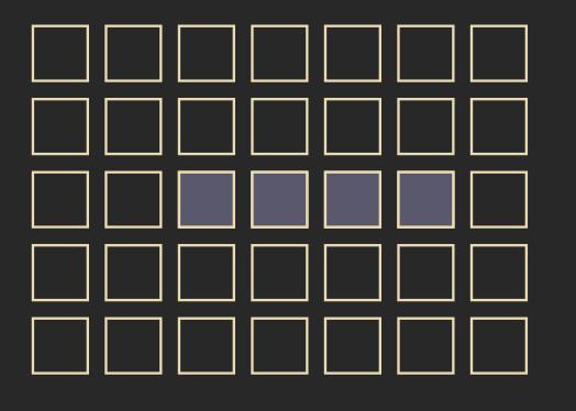
Example 3.9 – If we have a word of length \(n = 4\), the first four cells of our cellular automaton will contain the word, while the rest is filled with the resting state.

Example 3.10 – We want to use a cellular automaton to detect the formal language \(L = \{a\}^+\) with \(A = \{a, b\}\). This means the cellular automaton will receive inputs \(a\) and \(b\) and must detect words that consist only of the letter \(a\).
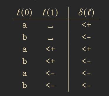
To solve this, we can simulate a finite state machine that accomplishes this. We choose the set \(C = \{0, 1\}\) and \(Q = \{a, b, <+, <-, \_ \}\).

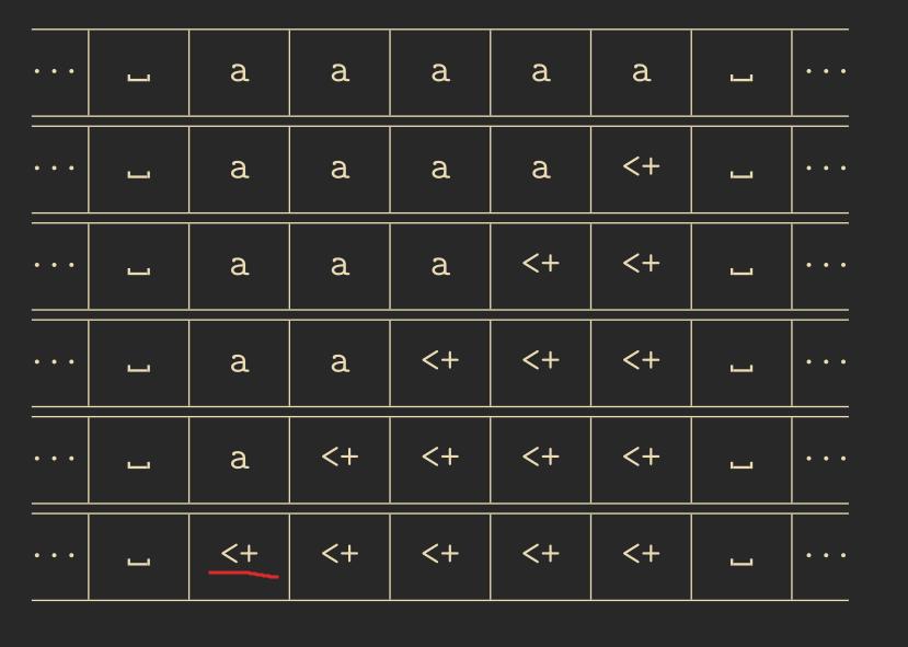
The above diagram is called a space-time diagram and is useful for visualizing multiple steps of a 1-dimensional cellular automaton.

The table below shows the transition function of the above cellular automaton. For cases not listed in the table, \(\delta(l) = l(0)\) applies.

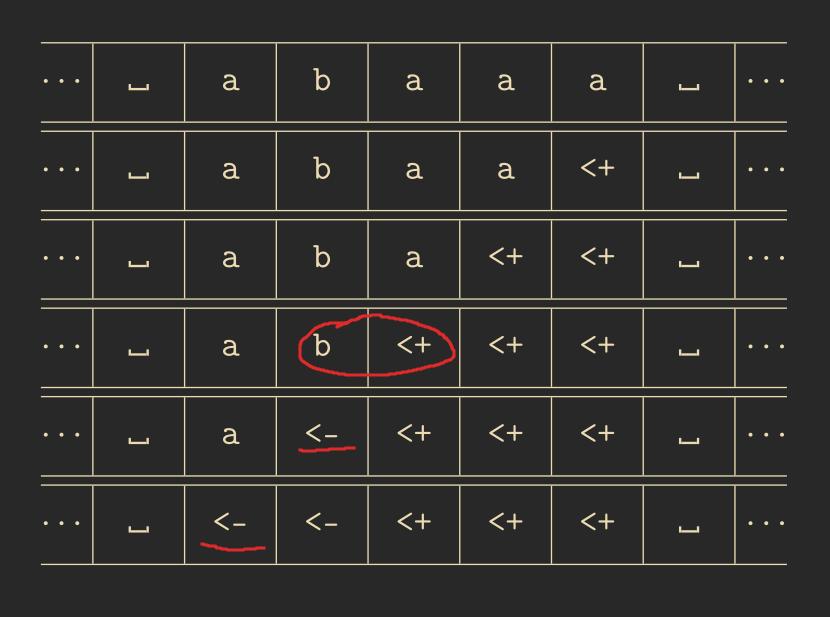
Example 3.11 – It is also possible to create a cellular automaton to detect all possible palindromes over a given alphabet, e.g., \(A = \{a, b\}\). Below is a space-time diagram for a negative example. The transition function is left out.

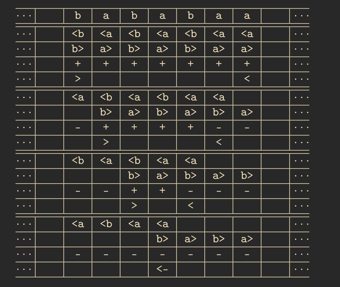
Do not be confused by the multiple lines. Per time step, as with the cellular automaton used to simulate the Turing machine, we use the Cartesian product to store multiple values in one cell.

4. Self reproduction

When John von Neumann first introduced CAs, one thing he was looking for was the ability of self-reproduction. This means that a CA with a pattern configuration \(c_m\) will, after some steps, reach a configuration where the pattern \(m\) appears several times.

Lemma 4.1 – Let \(p\) be a prime number, \(d\) the dimensionality, and \(N\) the neighborhood. For the CA \(C\) with \(R = \mathbb{Z}^d\), \(Q = \mathbb{Z}_p\), and \(\delta(l) = \sum_{n \in N} l(n) \mod p\), there exists, for any pattern \(m\), a \(k_0\) such that for all \(k > k_0\), the following holds true: After \(t = p^k\) steps, \(C\), starting from the configuration \(c_m\), reaches a configuration where the pattern \(m\) appears exactly \(|N|\) times.

The lemma above can be proven using the Multinomial theorem and induction.

Besides this CA, there are other constructions that can achieve self-reproduction, most notably the CA introduced in von Neumann’s book Theory of Self-Reproducing Automata.

5. Sorting with 1-dimensional CA

Problem Statement 5.1 – Let \(A = \{0,1\}\). We are searching for a CA with \(R = \mathbb{Z}\) that can take as input a pattern \(w \in A^+\) and transform it into the pattern \(0^{N_0(w)}1^{N_1(w)}\), where \(N_0(w)\) is the number of times the 0 appears in the pattern \(w\).

The above is the simplest formulation of the sorting problem; later, we will look at more complicated cases.

Algorithm 5.2 – We choose \(R = \mathbb{Z}, N = H_1^1, Q = A \cup \{\text{Rectangle}\}\) and define the transfer function as follows:

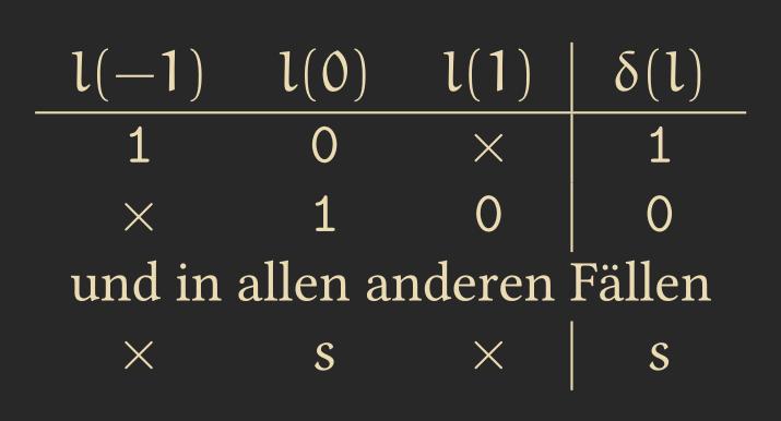
The transfer function switches a pair of \(01\) to \(10\) whenever it sees one. This means that in each step, at least one 1 and one 0 move closer to their end positions.

Unfortunately, we cannot generalize this algorithm to state sets with more than two numbers, e.g., \(\{0,1,2\}\), because we will always have some conflicts in the transfer function. For example, what should \(\delta(2,1,0)\) be? Should we switch the 2 with the 1 or the 1 with the 0?

One possible solution for this is to alternate looking left and right, which leads us to the Odd-Even-Transposition Sort.

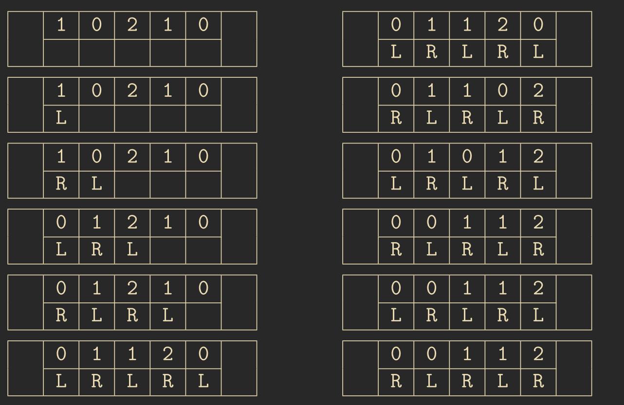
Odd-Even-Transposition Sort 5.3 – We again have a word consisting of numbers as input that we want to sort. This time, we have an additional space for each cell to indicate whether we want to look at this cell to the left or the right. Since this is not part of our input, we need to initialize these values ourselves. The transition function would be as follows, where \(s \in A\), \(x\) means that the state doesn’t matter, and \(\square\) means that the cell is empty:

\(l(-1)\)	\(l(0)\)	\(l(1)\)	\(\delta(l)\)
\((s, R)\)	\((t, L)\)	\(x\)	\((\max(s,t), R)\)
\(x\)	\((s, R)\)	\((t, L)\)	\((\min(s,t), L)\)
\(\square\)	\((t, L)\)	\(x\)	\((t, R)\)
\(x\)	\((s, R)\)	\(\square\)	\((s, L)\)

For the initialization of \(L, R\):

\(\square\)	\((s,\_)\)	\(x\)	\((s,L)\)
\((s,L)\)	\((s,\_)\)	\(x\)	\((s,R)\)

For all other cases:

x	z	x	z

Below is an example calculation with the Odd-Even-Transposition Sort CA:

An important lemma when attempting to prove the correctness of sorting algorithms is the following:

Lemma: Sorting from Knuth 5.4 – When a sorting algorithm consists only of operations of the type “compare and switch when bigger,” and when the starting input data and its positions remain fixed, then the following holds true: The algorithm sorts all input data correctly if and only if it sorts all input that consists solely of zeros and ones.

Using this lemma, one can easily prove the correctness of the Odd-Even-Transposition Sort algorithm.

6. Simple Techniques for CA

The first concept I want to introduce is signals. We’ve already encountered examples of them, for instance, the electron traveling through the wire in Wireworld.

Definition 6.1 – A signal is a mapping \(s: T \to R\), where \(T = \mathbb{N}\) represents a set of time stamps.

Thus, \(s(t)\) provides the position of the cell where the signal is located at time step \(t\).

Additionally, we want our signal to be constructible, meaning not all mappings defined above are feasible. This leads us to the next definition.

Definition 6.2 – A signal \(s\) is CA-constructible if a CA \(C\) exists such that, starting from the initial configuration \(c^0 : i \to s' \text{ if } i = s(0)\), the CA behaves so that for each configuration at time step \(c^t\), the following holds: \(c_{i+N}^t \iff s(t) = i\).

This means our signal is constructible if we have a starting configuration where the signal is present at the correct location, and in each subsequent timestep of our configuration, the signal remains at the appropriate location.

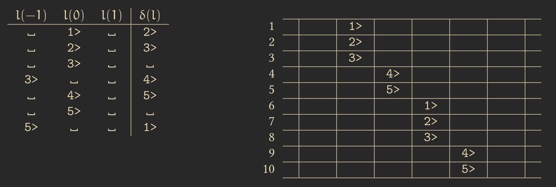
Algorithm: Signal with Constant Speed 6.3 – It is possible to construct a signal with a speed corresponding to any rational number \(r \in \mathbb{Q}\) with \( 0 < r < 1\). One such example is shown below for the case \(r = \frac{2}{5}\):

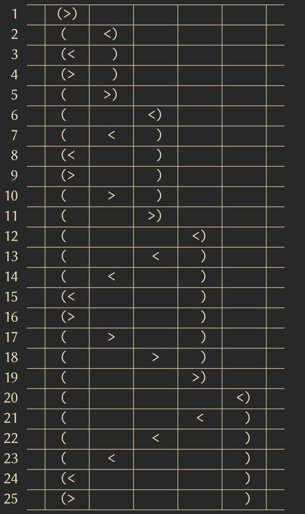
Algorithm: Parabolic Signal 6.4 – It is also possible to create signals with non-constant speeds. One such example is the Parabolic Signal, where three signals are used: the first signal always remains at the same position, the second signal bounces between the first and the third signal, and the third signal moves one cell to the left whenever it gets hit by the second signal. With this arrangement, the speed of the system continuously doubles. An example is shown below:

Definition 6.5 – A subset \(m \subset R \times \mathbb{N}_0\) is called a marking set.

Algorithm: Marking the Middle 6.6 – For example, we can use an algorithm to mark the midpoint between two points by sending two signals: one with speed \(\frac{1}{3}\) and the other with speed \(1\) in the same direction. The faster signal will reflect at the far end, and the signals will meet in the middle.

Definition 6.7 – We define the arrival time of a signal \(s\) as \(a_s : R \to T, x \mapsto \min\{t \mid s(t) = x\}\).

One interesting lemma related to this provides a lower bound on the speed a CA can achieve.

Lemma Veronique Terrier 6.8 – Let \(s\) be a constructible signal with monotonically increasing speed, and suppose we have a one-dimensional CA with an \(H_1^1\) neighborhood. Then, one of the following statements applies:
a) \(a_s(i) - i\) is constant.
b) \(\exists b \in \mathbb{N}_+ : a_s(i) - i \geq \log_b(i)\).

Besides signals, another useful tool in constructing a CA is counters. Below is the simplest implementation of one.

Algorithm: Walking Counter 6.9 – This algorithm realizes a counter through a one-dimensional CA that “walks”, incrementing by 1 with each step. The successive counter bits (with the least significant bit in front) in cell \(i\) represent the binary value of \(i\).

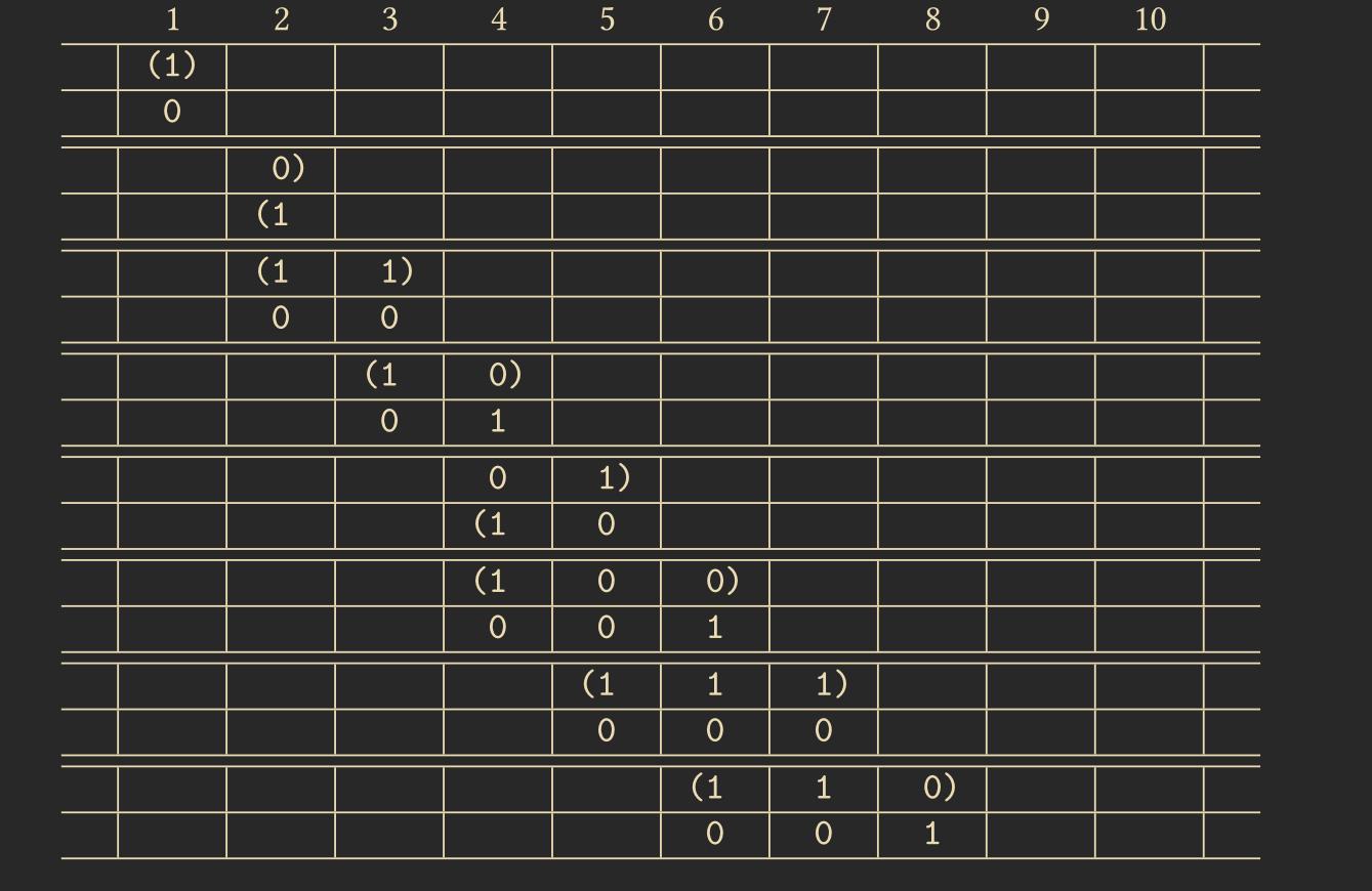
It is also possible to implement addition, multiplication, and division with CAs, though I will not cover them here.

7. Synchronisation

A good video introducing of this topic can be found here. The basic concept is that in cellular automata, all cells change their state simultaneously, which makes some algorithms difficult to implement when they require all cells to be synchronized. Thus, we want to find an algorithm that allows us to synchronize the cells.

Problem: Firing Squad Synchronization (FSSP) 6.10 – Given the state set \(Q' = \{\#, g, s, f\}\), we are searching for a CA \(C\) with a \(H_1^1\) neighborhood and state \(Q\), with \(Q' \subset Q\), that has the following properties:

• \(\{\#, s\}\) are passive states, with \(\#\) being the dead state.
• \(C\) transforms any configuration of the form \(c_g = \#gss...s\#\) into the configuration \(c_f = \#fff...f\#\) with the same number of cells.
• During the process, the state \(f\) must not appear in any configuration prior to the final configuration \(c_f\).

This problem must be solved by the CA regardless of the length of the starting configuration, meaning we cannot store the number of cells to be synchronized.

The state \(g\) represents the general, which is the leader initiating the synchronization process, while \(s\) represents the soldiers who must fire simultaneously. After firing, the soldiers enter the state \(f\).

Algorithm: Balzer 6.11 – The cell with \(1>>\) acts as the general. The main idea follows a divide and conquer approach by recursively dividing the space in half. To find the middle, we use the algorithm learned in the previous chapter. The recursion stops when the sections are small enough that each cell can detect its neighboring sections. The states \((\) and \()\) mark the synchronization sections, and the algorithm calculates subsequent sections recursively.

The overall running time of the algorithm is \(O(3n)\).

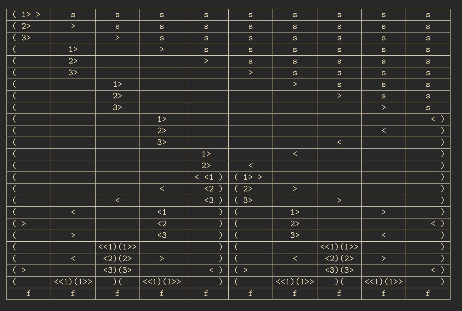
The following lemma provides a lower bound for the FSSP problem, meaning no algorithm can be faster than this.

Lemma: Waksman 6.12 – There is no CA that can solve the FSSP problem for a configuration of length \(n\) in fewer than \(2n - 3\) steps.

Several algorithms solve the FSSP problem optimally in exactly \(2n - 3\) steps, including those by Gerken 1987, Waksman, and Mazoyer 1987. These algorithms, instead of always dividing the space by a factor of 2, divide it into more sections, allowing for faster synchronization.

Problem: General at Arbitrary Position 6.13 – The next generalization of the FSSP problem is that the general is not always positioned on the left but instead can be randomly distributed in the starting configuration. The goal is to synchronize all the cells, regardless of the general’s position.

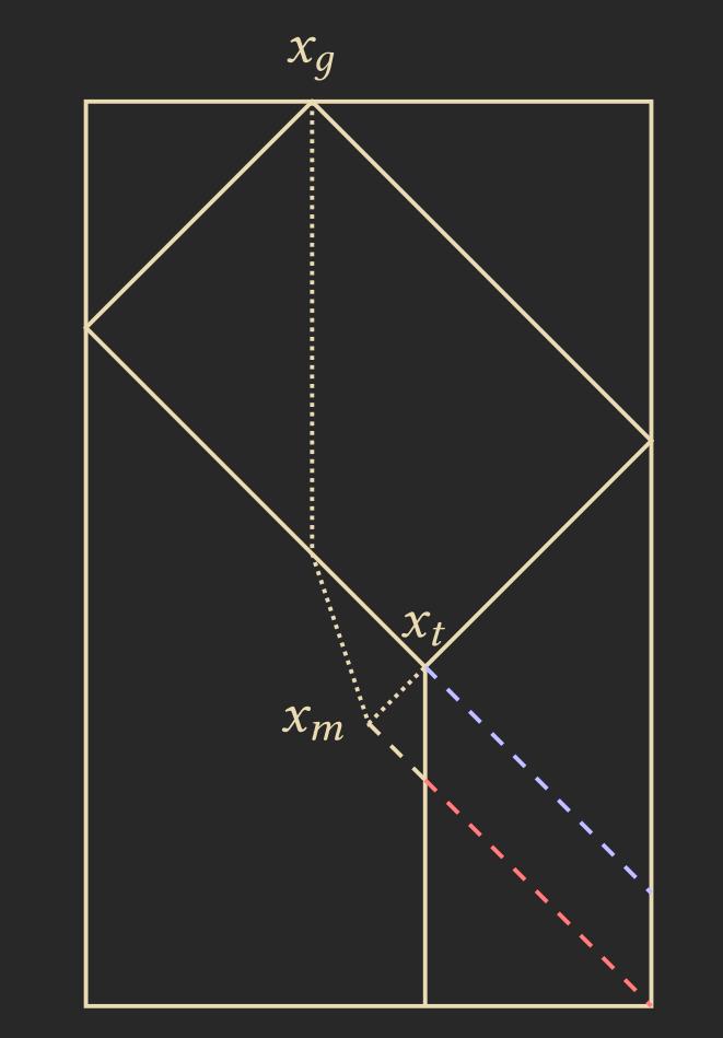
Algorithm: FSSP-1DIM-General-Arbitrary-Position 6.14 – Initially, the general is at position \(x_g\). We send a signal with speed 1 to both edges, starting the FSSP synchronization algorithm, whose area of effect reaches the position \(x_t\), where the reflected signals meet. This FSSP synchronization algorithm can be any of the previously mentioned ones, such as Balzer or Mazoyer.

In between some smaller sections, we need to freeze the algorithm to prevent it from advancing faster than the rest of the cells. We unfreeze these sections by sending a signal from the middle \(x_m\). We determine \(x_m\) using the middle-finding operation between \(x_g\) and \(x_t\).

Below is a sketch of the process, where the blue lines represent the freezing signal and the red lines represent the unfreezing signal:

Problem: Rectangle Synchronization 6.15 – So far, we have looked at synchronization in 1-dimensional space. But what if we want to synchronize a 2-dimensional space, such as a rectangle?

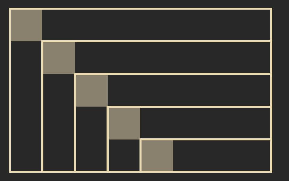
Algorithm: Synchronize Rectangle 6.16 – The rectangle consists of \(m\) rows and \(n\) columns. We assume the general is positioned at the 0-th row and 0-th column. We can use a slight modification of the FSSP-1DIM-General-Arbitrary-Position 6.14 algorithm to synchronize the rectangle. We start the algorithm by sending a signal with speed \(\frac{1}{3}\) from the general diagonally across the rectangle, triggering the synchronization process for the set \(M_i = \{(i,j) \mid j \geq i\} \cup \{(j,i) \mid j \geq i\}\). All \(M_i\) are synchronized at the same time.

In the sketch below, the \(M_i\) have the shape of a sideways “L”. We treat these “L"s or \(M_i\) as 1-dimensional synchronization cases, which we solve using the algorithm from 6.14.

This synchronization process can be further generalized to synchronize d-dimensional cuboids or even more complex, non-uniform d-dimensional shapes.

Another possible generalization would be to have no general at all, where the CA must elect a cell as the leader. This leads us to the Leader-Election Problem. There are CAs capable of solving this, but they are quite complex and won’t be covered here.

8. Sorting with 2-dimensional CA

Until now, we have only explored sorting in the 1-dimensional case. We now want to extend this to the 2-dimensional case, and for simplicity, we’ll limit ourselves to quadratic patterns. The first question we need to ask ourselves is: in what arrangement do we want to sort? Below, you can see some example arrangements, and for cellular automata, arrangement (c) is the easiest.

Problem: 2-dimensional Sorting 8.1 – I’ll leave out the formal problem definition, but generally, we have a chosen pattern \(e : \mathbb{N}_m \times \mathbb{N}_m \to A\) that we want to transform into a sorted pattern \(s : \mathbb{N}_m \times \mathbb{N}_m \to A\) with certain properties.

Algorithm: Shear Sort 8.2 – The algorithm works in \(1 + \log(m)\) phases. In phases \(1, 3, 5, ..., 1 + \log(m)\), we sort each row individually. For instance, we can use the odd-even transposition sort (5.3) here, sorting the odd-numbered rows in ascending order from left to right and the even-numbered rows in ascending order from right to left.

In phases \(2, 4, 6, ..., 2\log(m)\), we sort each column, moving the smaller values toward the top.

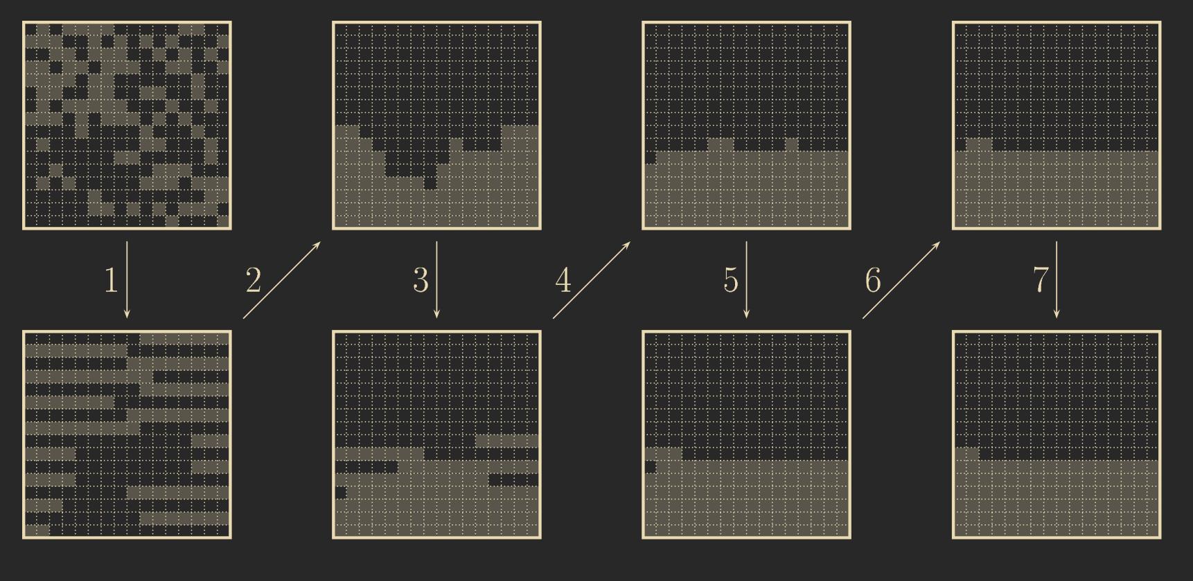
For this algorithm to work, we first need a phase \(0\), where all cells are initialized with the information on whether they are in an odd or even-numbered row, allowing them to sort accordingly.

This initialization can be done for each column starting from the top row, taking \(m\) steps (the number of cells in a row) by walking a modulo-2 counter downward for each column. Simultaneously, we can run a FSSP algorithm that ends at the same time and initiates the sorting process once the initialization is complete. To switch the sorting behavior between odd and even rows, we can again use a FSSP algorithm to toggle the behavior after \(m\) steps (since it takes \(m\) steps for odd-even transposition sort to sort one row).

Lemma 8.3 – The Shear Sort algorithm produces a sorted pattern for all input configurations and takes \(O(\sqrt{n}\log(n))\) steps.

It is important to note that the correctness of the Shear Sort algorithm is not trivial. For example, if you change the direction so that both odd and even rows sort in the same way, the algorithm will no longer work.

To prove the correctness of Shear Sort, the Knuth Sorting Lemma (5.4) can be used.

There is another algorithm for 2-dimensional sorting by Schnorr and Shamir, where the input quadratic pattern is divided into four equally-sized quadrants. It runs 9 distinct phases, each doing something different. I won’t go into much more detail, but the algorithm has a running time of \(O(\sqrt{n})\).

Lemma 8.4 – Any algorithm for 2-dimensional sorting in serpentine line form for CA requires at least \(3\sqrt{n} - o(\sqrt{n})\) steps if it needs to sort an arbitrary number of values.

An interesting takeaway is that using CA, we can apply odd-even transposition sort to sort in \(O(n)\), and we can use the Schnorr and Shamir algorithm to sort in 2 dimensions in \(O(\sqrt{n})\). Both are more efficient than their classical non-CA sorting algorithm counterparts.

9. Asynchronous CA

We’ve seen many different CAs and algorithms so far, but they all had one commonality: all the cells change deterministically and synchronously. However, this is not always achievable. One could imagine that in the future, CAs could be used for nanotechnology, with tiny robots injected into the bloodstream to unclog arteries or repair cell damage. But one problem arises—synchronizing these tiny robots. To synchronize, they need to emit signals to communicate with each other. However, because they are so small, this might not be possible, or they may only have weak transmitters that allow occasional communication. For certain applications, such as simulating natural phenomena, asynchronous CAs might also provide more realistic results.

As such, we want to explore asynchronous CAs, where not all cells update simultaneously.

Definition: Asynchronous CA 9.1 – Asynchronous mode of operation:

• Subset \(A \subset R\) of active cells
• \(F_A : Q^R \to Q^R\) induced by \(f\) according to
  • Active cells: \(\forall x \in A : F_A(c)(x) = f(L(c,x))\)
  • Passive cells: \(\forall x \in R \backslash A : F_A(c)(x) = c(x)\)
• \(F_A\) is a function.

This means that we have a certain subset of our space that consists of active cells, and these change their state according to the transfer function \(F_A\). All other cells that are not active do not change their state but instead keep their current state. This set of active cells doesn’t need to be fixed and can change over time.

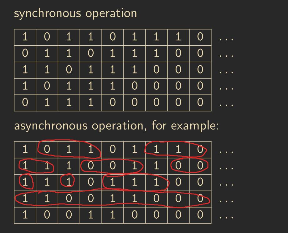
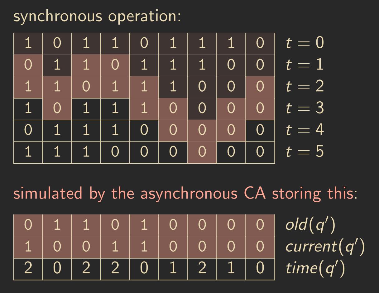
Example: Rule 170 9.2 – The CA Rule 170 has the transfer function \(f(l) = l(1)\), i.e., we shift all states one to the left per step. An example can be seen in the space-time diagram below. The red-marked cells are the active cells:

Algorithm: Nakamura (1970) 9.3 – We now have an asynchronous CA and want to use it to simulate a synchronous CA so that we can apply already learned synchronous algorithms to our asynchronous CA. The idea is to let some cells be ahead of others but never more than one step compared to any other cell in the neighborhood, and to remember the old state for those behind.

We will set the state set to \(Q' = Q \times Q \times \{0,1,2\}\), where the first \(Q\) stores the current state of the cell, the second \(Q\) stores the state from the last step, and \(\{0,1,2\}\) tracks how far ahead the cell is. We can then define our transfer function as follows:

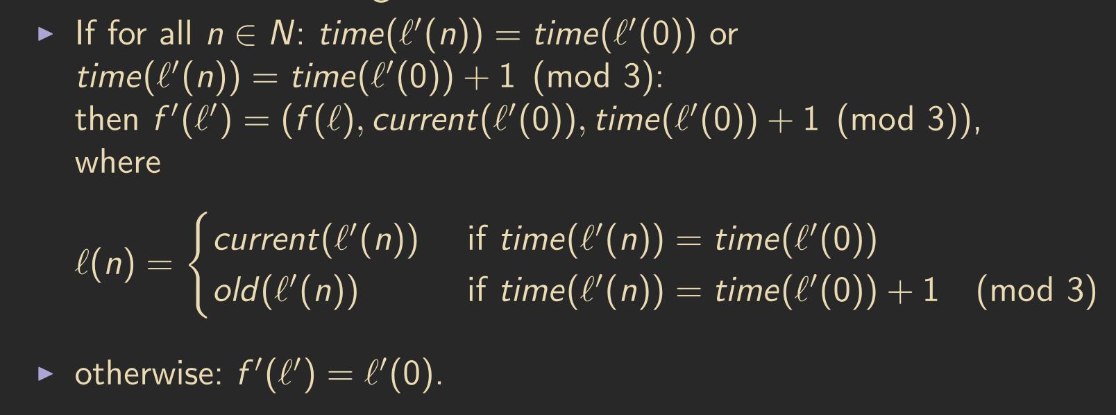
This “if” statement means that the time of the cells in the neighborhood needs to be the same or at most one step ahead for the transfer function to work. If this is not the case, the cells are not allowed to change their state, giving the other cells time to catch up.

Example: Rule 170 9.4 – We again look at the CA Rule 170, but this time we use the Nakamura technique to simulate a synchronous CA using an asynchronous CA.

Definition: \(\alpha\)-Asynchronous CA 9.5 – Instead of choosing the active cells deterministically, we now want to randomly select which cells are active and which are passive. We introduce \(\alpha\), a probability between 0 and 1, and make the set of active cells \(A\) a random variable. Our CA behaves as follows:

• In each step, each cell \(x\) is included in \(A\) with a probability \(\alpha\), independently of the others.
• After we have chosen \(A\), we use the transfer function \(F_A\) to update the cells, then restart the process.

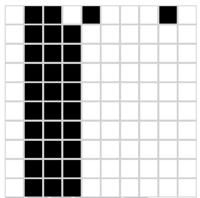
Example: Majority Rule (232) 9.6 – We set our transfer function as follows:

\[ f(l) = \begin{cases} 0, \ \text{if } l(-1) + l(0) + l(1) \leq 1\\ 1, \ \text{if } l(-1) + l(0) + l(1) \geq 2 \end{cases} \]

With synchronous updating, blocks of at least two consecutive bits are conserved, and isolated bits are destroyed. When using asynchronous updating with a small \(\alpha\), it takes some time for the isolated bits to be destroyed.

Example: Traffic Rule (184) 9.7 – A “car,” marked by the state “1,” moves to the right if there is an “empty street” marked by state “0,” leaving an “empty street” behind. Otherwise, the “car” stays where it is. The total number of 0s and 1s never changes.

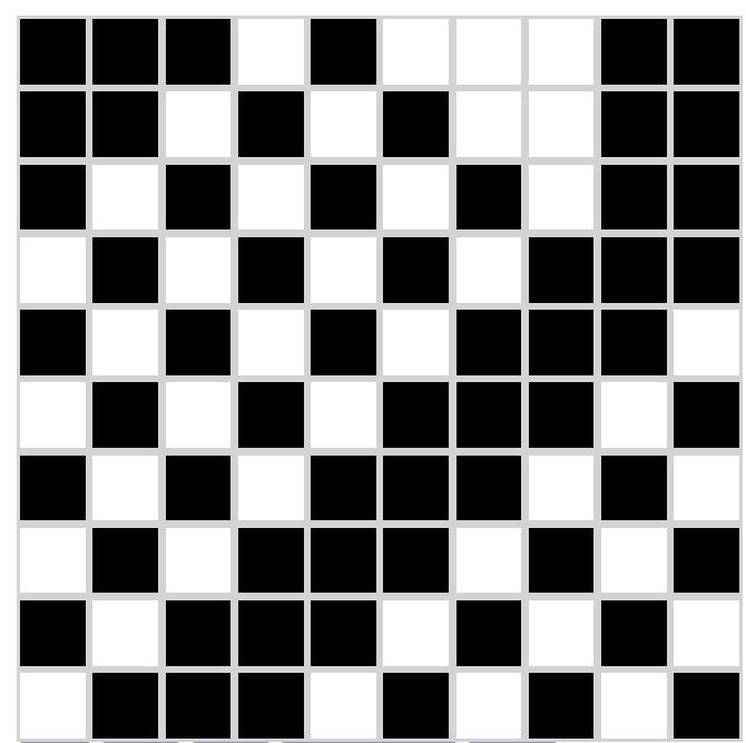
With synchronous updating, separated cars move to the right, and traffic jams move to the left. When using asynchronous updating with a very large \(\alpha\), basically the same thing happens.

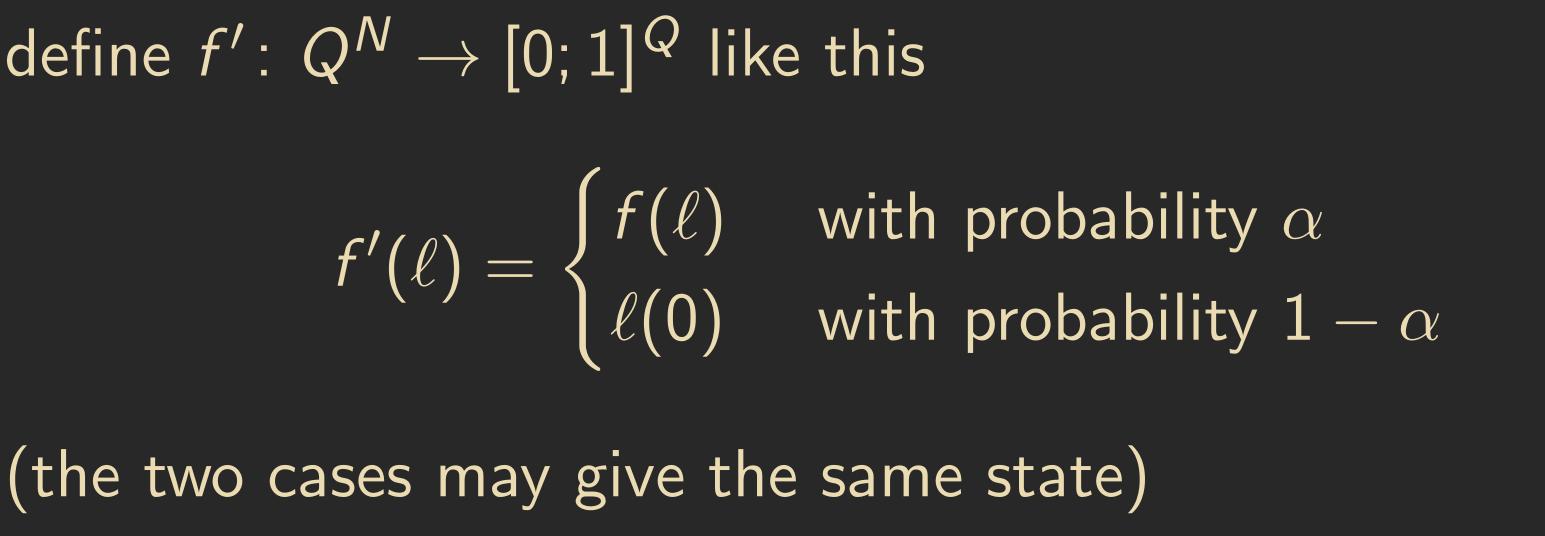
Definition 9.8 – We now define a probabilistic CA. The local transfer function is \(f: Q^N \to [0,1]^Q\), where \(f(l)(q)\) is the probability that a cell observing \(l\) in its neighborhood chooses \(q\) as its new state. For this function to make sense, we have an additional requirement \(l \in Q^N : \sum_{q \in Q} f(l)(q) = 1\). \(f\) is applied using synchronous mode of operation.

In fact, it turns out that \(\alpha\)-asynchronous CAs are a special case of probabilistic CAs with the following transfer function:

Problem 9.9 – We have an initial configuration \(c_s\), where cells have either the state \(0\) or \(1\). The goal is to find an algorithm that results in a final configuration \(c_f\), where all cells have the state \(0\) if \(c_s\) contains more cells with state \(0\) than state \(1\). Otherwise, all cells should have the state \(1\). This problem is called density classification.

Theorem: Land/Belew (1995) 9.10 – There is no deterministic CA that can solve the density classification problem with synchronous updating.

Algorithm: Fuks (1995) 9.1 – The density classification problem can be solved using two CAs:

• First, run \(n/2\) steps with Rule 184 (traffic rule).
• Then, run \(n/2\) steps with Rule 232 (majority rule).

Algorithm: Fates (2011) 9.2 – The density classification problem can be solved using a probabilistic CA with the following local transfer function:

\[ f(l) = \begin{cases} f_{184}(l), \text{with probability } \alpha \\ f_{232}(l), \text{with probability } 1 - \alpha \end{cases} \]

Where \(\alpha\) needs to be sufficiently large.

10. Conclusion

That’s it. I hope you’ve learned a thing or two! The field of cellular automata is much broader than what I’ve covered here. If you’re interested in diving deeper, I can recommend a few topics: the Abelian sandpile model, Algorithms for Leader Election by Cellular Automata, Block cellular automaton, Lattice gas automaton, and the Nagel–Schreckenberg model, just to name a few.

---

References:

• This article is based on the lecture “Algorithms in Cellular Automata” by Thomas Worsch.