Lets Program LeNet
November 6, 2024 | 1,941 words | 10min read
LeNet is one of the first convolutional neural networks (CNNs). Its design is relatively simple and well-documented, making it a good candidate for implementation to gain practice with a deep learning library such as PyTorch.
In this article, I will show how you can use PyTorch to implement a deep convolutional neural network, train it, and perform inference. If you are interested in more of the theory, I recommend consulting my prior post on CNNs. Another excellent resource is the CS231n site on CNNs.
Familiarity with how convolutional neural networks work is recommended, as this article focuses mainly on the practical side.
Prerequisites
You will need an up-to-date Python version installed. Additionally, you will need to install PyTorch, a deep learning library, and torchvision, which provides datasets for testing. To install PyTorch and torchvision, I recommend using Conda, which allows you to create a virtual Python environment where libraries won’t conflict with others you have installed. (If you are familiar with Docker, it is similar but specific to Python.) Alternatively, you can use pip, Python’s default package manager.
Run the command from the PyTorch site in the terminal to get started. If you have an NVIDIA GPU with CUDA installed, you can use the CUDA version, which allows PyTorch to take advantage of your GPU for faster training and inference. Otherwise, use the CPU version.
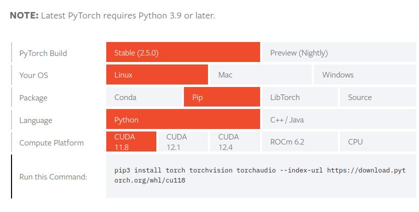
When installing PyTorch with CUDA, it is important to select the compatible CUDA version. If you have CUDA installed but are unsure of your version, you can use the following command to check:
1nvcc --version
If CUDA is not installed on your system, refer to NVIDIA’s official installation guide.
In addition to PyTorch, we will use Matplotlib for visualization purposes. Refer to their installation guide if you need help with installation.
LeNet Overview
First, we need to clarify the components that make up LeNet-5. Below is a visualization of its architecture.
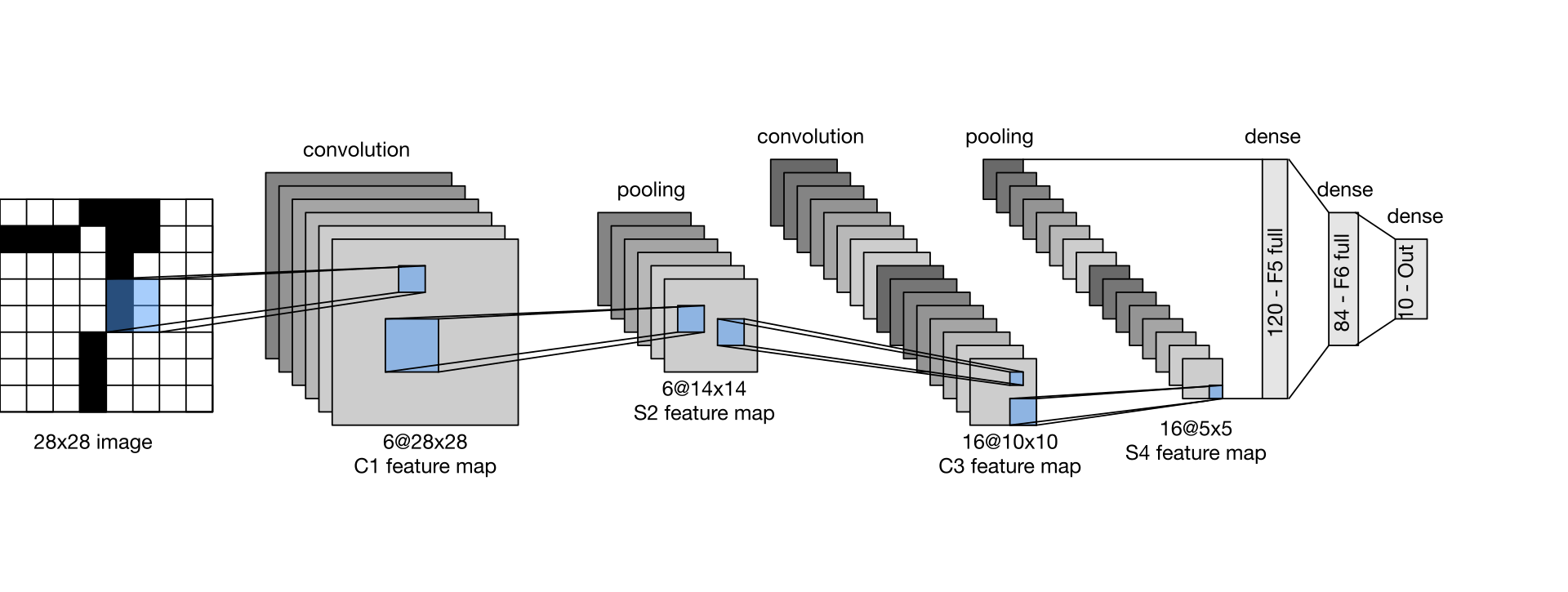
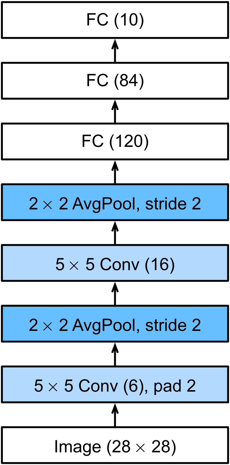
As shown, LeNet-5 consists of three main components:
- Convolutional layer, which uses a 2-dimensional kernel to scan the input from the previous layer.
- Linear layer, also called dense or fully connected layers.
- Pooling layer, specifically an average pooling layer, which is mainly used to reduce dimensionality.
Each of these layers has additional attributes, known as hyperparameters, that can be identified from the block diagram.
The input layer expects an input size of 28x28. The first convolutional layer will have 6 feature maps (output channels), with a kernel size of 5x5 and 2 pixels of padding. The average pooling layer will use a kernel size of 2x2 with a stride of 2.
A brief explanation, Kernel size refers to the dimensions of the filter (e.g., 3x3 or 5x5) used in a convolutional layer to scan the input image or feature map. Stride defines how many pixels the filter moves across the input during each convolution operation, affecting the output size. And at last, Padding involves adding extra pixels (usually zeros) around the input image to ensure the filter can fully cover the edges of the input or to control the output size.
Implementation of LeNet
Now that we know the specific hyperparameters of our model, we can start coding. First, we need to define the structure of our network. PyTorch provides the Module class, which our neural network should inherit from. This setup will make it easier to train our network later.
Let’s import some of the libraries we’ll use:
1# Importing all the libraries we need for now
2import torch
3import torch.nn as nn
4import torch.nn.functional as F
Next, we can define our PyTorch Module class:
1# Our neural network
2class LeNet(nn.Module):
3    def __init__(self):
4        super(LeNet, self).__init__()
5        pass
6
7    def forward(self, x):
8        pass
In the constructor (__init__), we’ll define the layers of our network. The forward method specifies what the network should do during the forward pass—in other words, how the layers should be applied to our input.
Let’s define our first convolutional layer. It has one input channel, because our input will be grayscale images (with only one color channel), 6 output channels, and a kernel size of 5:
1self.conv1 = nn.Conv2d(1, 6, 5)
The pooling layer is similarly easy to define; we just need to pass the kernel size and then the stride:
1self.pool1 = nn.AvgPool2d(2, 2)
For the fully connected (linear) layer, we specify the number of input neurons and output neurons:
1self.fc1 = nn.Linear(400, 120)
You might wonder how to determine the 400 input neurons, given that only the output neurons are displayed in the LeNet block diagram. There are two ways:
- You can calculate it using the formula below: \[ H_{\text{out}} = \lfloor \frac{H_{\text{in}} + 2 \times \text{padding} - \text{kernelsize} - 1}{\text{stride}} + 1 \rfloor \]
- Alternatively, set it to a random value and add a print statement before the linear layer definition to print the data’s dimensions.
With this knowledge, we can now define all the layers of our CNN:
 1class LeNet(nn.Module):
 2    def __init__(self):
 3        super(LeNet, self).__init__()
 4
 5        self.conv1 = nn.Conv2d(1, 6, 5)
 6        self.pool1 = nn.AvgPool2d(2, 2)
 7        self.conv2 = nn.Conv2d(6, 16, 3)
 8        self.pool2 = nn.AvgPool2d(2, 2)
 9
10        self.fc1 = nn.Linear(400, 120)
11        self.fc2 = nn.Linear(120, 84)
12        self.fc3 = nn.Linear(84, 10)
Then, we can define the forward method, which processes the input through each layer:
 1    def forward(self, x):
 2        x = self.conv1(x)
 3        x = F.relu(x)
 4        x = self.pool1(x)
 5
 6        x = self.conv2(x)
 7        x = F.relu(x)
 8        x = self.pool2(x)
 9
10        # Uncomment the line below to print the dimensions of the data
11        # print(x.size())
12
13        # Flatten the 2D data to 1D
14        x = x.view(-1, 400)
15
16        x = self.fc1(x)
17        x = F.relu(x)
18
19        x = self.fc2(x)
20        x = F.relu(x)
21
22        x = self.fc3(x)
23
24        return x
Testing our Model on the MNIST Datast
To test our model, we will use images from the MNIST dataset, a widely used collection of grayscale, handwritten digits. This dataset serves as a benchmark for evaluating image classification models, as it provides simple, standardized images that help assess how well the model recognizes basic patterns.
We can load this dataset using PyTorch’s DataLoader class from the torchvision library. We’ll also apply normalization to scale the pixel values. The values for normalization are sourced from this discussion:
 1import torchvision
 2import time
 3
 4test_transform = torchvision.transforms.Compose([
 5    torchvision.transforms.ToTensor(),
 6    torchvision.transforms.Normalize((0.1307,), (0.3081,))
 7])
 8
 9train_transform = torchvision.transforms.Compose([
10    torchvision.transforms.ToTensor(),
11    torchvision.transforms.Normalize((0.1307,), (0.3081,))
12])
13
14test_loader = torch.utils.data.DataLoader(
15    torchvision.datasets.MNIST(
16        '.',
17        train=False,
18        download=True,
19        transform=test_transform
20    ),
21    batch_size=64,
22    shuffle=False,
23    drop_last=True
24)
25
26train_loader = torch.utils.data.DataLoader(
27    torchvision.datasets.MNIST(
28        '.',
29        train=True,
30        download=True,
31        transform=train_transform
32    ),
33    batch_size=64,
34    shuffle=False,
35    drop_last=True
36)
We can view a sample image from this dataset using the matplotlib library. The following code loads and displays a sample image from the dataset using matplotlib, applying a grayscale colormap and no interpolation.
1import matplotlib.pyplot as plt
2
3sample = next(iter(train_loader))[0][0].squeeze()
4
5plt.imshow(sample, cmap='gray', interpolation='none')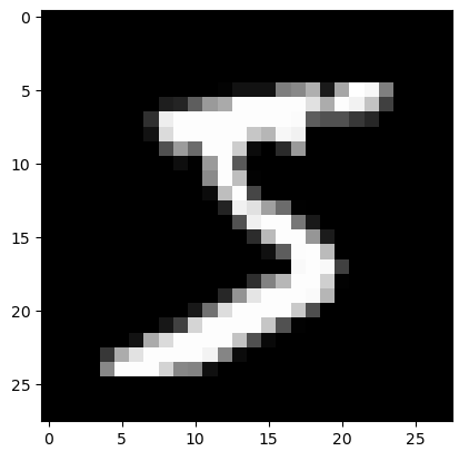
Once we initialize our model, we can pass this image through our network to see what digit the model predicts:
1net = LeNet()
2
3sample = next(iter(train_loader))[0][0]
4net.forward(sample)
This produces the following output:
1tensor([[-0.0340, 0.0443, -0.0341, -0.0727, 0.0751, 0.0734, 0.0544, -0.0317, 0.0051, -0.1094]], grad_fn=<AddmmBackward0>)
The higher each value is, the more likely the model thinks that the index of that value corresponds to the digit in the image. To get the actual prediction of the digit, we need to take the argmax of the output tensor:
1torch.argmax(torch.tensor([[-0.0340, 0.0443, -0.0341, -0.0727, 0.0751, 0.0734, 0.0544, -0.0317, 0.0051, -0.1094]]))
This returns torch.tensor(7), meaning the model predicts that the digit in the image is 7.
As you can see from the image we depicted earlier, the initial prediction is not accurate. This is expected, as we haven’t yet trained our network. To improve its performance, we will implement a training routine for our model.
Training our LeNet Model
To train our model, we first define the number of epochs, which represents how many times we want to iterate over the entire training dataset. Next, we set up the loss function, which measures how close the model’s predictions are to the actual target values. For this, we use cross-entropy loss, a standard for classification problems. Additionally, we define an optimizer, which is responsible for adjusting the model parameters to minimize the loss. Here, we’ll use stochastic gradient descent (SGD), but you could also experiment with other popular optimizers, such as Adam:
1n_epochs = 5
2
3optimizer = torch.optim.SGD(net.parameters(), lr=0.01)
4# optimizer = torch.optim.Adam(net.parameters(), lr=0.1)
5loss_function = nn.CrossEntropyLoss()
We also need to specify the device on which we want to perform the computations, either the cpu or cuda (if a compatible GPU is available):
1net = LeNet()
2
3device = torch.device('cpu')
4net.to(device)
Next, we iterate over our dataset in batches. The batch size, which we specified earlier in the train_loader, determines the number of images processed at once:
1for epoch_n in range(n_epochs):
2    for batch_idx, (inputs, targets) in enumerate(train_loader):
3        pass
Within this loop, we perform the actual training. We start by clearing any gradients saved from previous iterations with optimizer.zero_grad() and transferring both inputs and targets to the device:
1optimizer.zero_grad()
2inputs, targets = inputs.to(device), targets.to(device)
We then compute the model’s predictions by passing the inputs through the network. To calculate the loss, we compare these predictions with the actual targets using our loss function:
1preds = net(inputs)
2loss = loss_function(preds, targets)
The final steps involve backpropagating the loss and updating the model’s parameters:
1loss.backward()
2optimizer.step()
To monitor the training process, we can calculate the accuracy and store both the loss and accuracy values over each epoch:
1# Calculate accuracy
2predicted_labels = torch.argmax(preds, dim=1)
3correct = (predicted_labels == targets).sum().item()
4accuracy = correct / targets.size(0)
5
6loss_tmp.append(loss.item())
7acc_tmp.append(accuracy)
With these steps, we can now train our model. The complete training loop is as follows:
 1net = LeNet()
 2device = torch.device('cpu')
 3
 4optimizer = torch.optim.SGD(net.parameters(), lr=0.01)
 5loss_function = nn.CrossEntropyLoss()
 6
 7n_epochs = 5
 8loss_list = []
 9acc_list = []
10
11for epoch_n in range(n_epochs):
12    loss_tmp = []
13    acc_tmp = []
14
15    for batch_idx, (inputs, targets) in enumerate(train_loader):
16        optimizer.zero_grad()
17        inputs, targets = inputs.to(device), targets.to(device)
18
19        preds = net(inputs)
20
21        # Calculate loss
22        loss = loss_function(preds, targets)
23        loss.backward()
24        optimizer.step()
25
26        # Calculate accuracy
27        predicted_labels = torch.argmax(preds, dim=1)
28        correct = (predicted_labels == targets).sum().item()
29        accuracy = correct / targets.size(0)
30
31        loss_tmp.append(loss.item())
32        acc_tmp.append(accuracy)
33
34        if batch_idx % 100 == 0 and batch_idx != 0:
35            l_avg = sum(loss_tmp) / len(loss_tmp)
36            a_avg = sum(acc_tmp) / len(acc_tmp)
37
38            print(f"Epoch [{epoch_n+1}/{n_epochs}], Batch [{batch_idx // 100}], Avg Loss: {l_avg:.4f}, Avg Acc: {a_avg:.4f}")
39
40            loss_list.append(l_avg)
41            acc_list.append(a_avg)
Plotting the Accuracy and Loss of Training
We can plot the loss and accuracy of the training process using the matplotlib library to ensure that the training is progressing correctly. Here’s how you can visualize the training metrics:
 1import matplotlib.pyplot as plt
 2import numpy as np
 3
 4plt.rcParams['figure.figsize'] = [10, 5]
 5
 6fig, ax = plt.subplots(1)
 7
 8# Plot accuracy
 9ax.plot(np.array(acc_list), color='tab:blue')
10ax.set_xlabel('Mini-batch steps (100)')
11ax.set_ylabel('LeNet Accuracy')
12ax.tick_params(colors='tab:blue', axis='y')
13
14# Plot loss
15ax2 = ax.twinx()
16ax2.plot(np.array(loss_list), color='tab:red', label='Loss')
17ax2.set_ylabel('LeNet Loss')
18ax2.tick_params(colors='tab:red', axis='y')
19
20ax.set_title('LeNet Training')
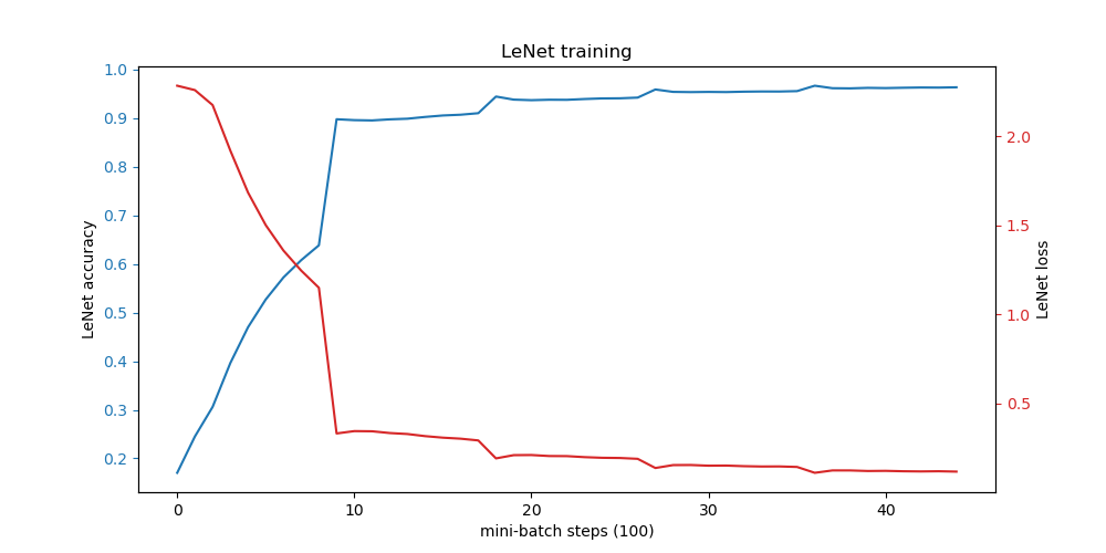
After training, when we pass an image through the model again, it now correctly predicts the number in the image:
1torch.tensor(5)
Conclusion
With this, you’ve seen a basic implementation of LeNet, one of the first Convolutional Neural Networks (CNNs). There are many improvements that can be made on top of it, as demonstrated in more advanced architectures like ResNet, InceptionNet, and DeformableNet just to name a few.
