Numerical Methods for Computer Scientist
September 21, 2025 | 22,294 words | 105min read
The following is a sheet of numerical problems and their solutions. It is a mix of problems taken from old exams and practice sheets from the KIT "Numerische Mathematik für die Fachrichtungen Informatik" lecture. This is similar to the article Optimization Problem, but for numerical problems instead.
Problems with Confirmed Solution
This section contains only problems with official solutions.
Problem 1: Floating Point Arithmetic
We consider for a given base \( B \geq 2 \), a minimum exponent \( E^{-} \), and lengths \( M \) and \( E \), the finite set of normalized floating-point numbers \(\text{FL}\).
\[ \text{FL} := \left\{ \pm B^e \sum_{l=1}^M a_l B^{-l} : e = E^{-} + \sum_{k=0}^{E-1} c_k B^k, a_l, c_k \in \{0, \ldots, B - 1\}, a_1 \neq 0 \right\} \cup \{0\} \]Let \( E^{+} \) be the maximum exponent, \( m \neq 0 \) the mantissa, \( \max \text{FL} \) the largest number of the set, and \( \min \text{FL}_+ \) the smallest positive number of the set.
a) Show that:
(i) \( E^+ = E^{-} + B^E - 1 \) (ii) \( B^{-1} \leq |m| < 1 \) (iii) \( \max \text{FL} = -\min \text{FL} = B^{E^+}(1 - B^{-M}) \) (iv) \( \min \text{FL}_+ = B^{E^{-} - 1} \)
b) Calculate for the IEEE Standard of
- single precision \((B = 2, E^{-} = -126, M = 23, E = 8)\)
- double precision \((B = 2, E^{-} = -1022, M = 52, E = 11)\)
the values for \( E^+ \), \( \max \text{FL} \), \( \min \text{FL}_+ \), and the machine epsilon \( \varepsilon \).
c) Reformulate
\[ f(x) = \sqrt{x + \frac{1}{x}} - \sqrt{x - \frac{1}{x}} \quad \text{for } |x| \gg 1 \]in such a way that cancellation is avoided. Determine the absolute condition number of \( f \) at the point \( x = 100 \) before and after the transformation. Hint: For evaluating the derivatives, we recommend using digital tools.
Solution a)
(i)
$$ \begin{align*} e_{max} &= e_{min} + \sum_{i = 0}^{L_e -1 } (B-1) B^l \\ &= e_{min} + (B-1) \sum_{i = 0}^{L_e -1 } B^l \\ &= e_{min} + (B-1) \frac{1-B^L_e}{1 - B} \\ &= e_{min} - (B-1) \frac{1-B^L_e}{B - 1} \\ &= e_{min} - (1-B^L_e) \\ &= e_{min} + B^{L_e} - 1 \end{align*} $$(ii)
$$ \begin{align*} |m| &= |\sum_{l = 1}^{M} a_l B^{-l}| \\ &\geq | 1 \cdot B^{-1}| \\ &\geq B^{-1} \\ \\ |m| &= |\sum_{l = 1}^{M} a_l B^{-l}| \\ &\leq (B -1 ) \sum_{l = 1}^{M} B^{-l} \\ &= (B -1 ) \sum_{l = 0}^{M-1} B^{-1} B^{-l} \\ &= (B - 1) (B^{-1}) \frac{1 - B^{-M}}{1 - B} \\ &= (B - 1) (B^{-1}) \frac{1 - B^{-M}}{-(B-1)} \\ &= \frac{1 - B^{-M}}{-B} \\ &\leq 1 \end{align*} $$(iii)
$$ \begin{align*} -minFL = maxFL =^{(ii)} B^{E^+}(B^{-M} - 1) \end{align*} $$(iv)
$$ \begin{align*} minFL_+ = B^{e_{min}}B^{-1} = B^{e_{min} - 1} \end{align*} $$Solution b)
For eps we have:
For single precision:
- \(E^+ = -126 + 2^8 -1 = 129\)
- \(maxFL = 2^{129}(1 - 2^{-52}) = 6.8 * 10^{38}\)
- \(minFL_+ = 2^{-126 -1} = 5.8 * 10^{-39}\)
- \(eps = 1.10 * 10^{-7}\)
For double precision:
- \(E^+ = 1025\)
- \(maxFL = 3.6 * 10^{308}\)
- \(minFL_+ = 1.1* 10^{-308}\)
- \(eps = 2.2 * 10^{-16}\)
Solution c)
$$ \begin{align} f(x) &= \sqrt{x + \frac{1}{x}} - \sqrt{x - \frac{1}{x}} \\ &= \left(\sqrt{x + \frac{1}{x}} - \sqrt{x - \frac{1}{x}}\right) \frac{\sqrt{x + \frac{1}{x}} + \sqrt{x - \frac{1}{x}}} {\sqrt{x + \frac{1}{x}} + \sqrt{x - \frac{1}{x}}} \\ &= \frac{2}{x(\sqrt{x + \frac{1}{x}}) + \sqrt{x + \frac{1}{x}})} \\ &= \hat{f}(x) \end{align} $$We can then calculate the derivative of \(f(x)\) and \(\hat{f}(x)\) the absolute condition number is then the absolute value of the derivative.
$$ |f'(100)| = 0.000015 = |\hat{f}(100)| $$Problem 2: LR-Decomposition
Let \(\alpha \in \mathbb{R} \setminus \{0\}\), \(\beta, \gamma, \delta \in \mathbb{R}\) and
$$ A = \begin{pmatrix} \alpha & \beta \\ \gamma & \delta \end{pmatrix}. $$a) Derive the LR-decomposition \(A = LR\).
Now let specifically \(\alpha > 0\), \(\beta = \gamma = 1\) and \(\delta = 0\).
b) Determine the condition of \(A, L\) and \(R\) with respect to \(\| \cdot \|_1, \| \cdot \|_\infty\) and \(\| \cdot \|_F\) as an estimate of the spectral norm.
c) Compare how, for an arbitrary right-hand side \(\mathbf{b} \in \mathbb{R}^2\) and \(|\alpha| \ll 1\), the solutions of the equations
$$ A\mathbf{x}^1 = \mathbf{b}, \quad L R \mathbf{x}^2 = \mathbf{b} $$react to a relative perturbation of the right-hand side of 10%.
Solution a)
We want to find a matrix \(R\) and \(L\) so that
$$ A = LR $$with
$$ L = \begin{pmatrix} 1 & 0 \\ l_{21} & 1 \end{pmatrix} \quad R = \begin{pmatrix} r_{11} & r_{12} \\ 0 & r_{22} \end{pmatrix} $$Thus we get:
$$ \begin{align} \alpha &= r_{11} \\ \beta &= r_{12} \\ \gamma &= l_{21} r_{11} \\ \delta &= l_{21} r_{12} + r_{22} \end{align} $$which is the same as:
$$ \begin{align} \alpha &= r_{11} \\ \beta &= r_{12} \\ \gamma &= l_{21} \alpha \\ \delta &= l_{21} \beta + r_{22} \end{align} $$Hence
$$ \begin{align} \alpha &= r_{11} \\ \beta &= r_{12} \\ l_{21} &= \frac{\gamma}{\alpha} \\ r_{22} &= \delta - l_{21}\beta = \delta - \frac{\gamma\beta}{\alpha} \end{align} $$So our final decomposition is
$$ L = \begin{pmatrix} 1 & 0 \\ \frac{\gamma}{\alpha} & 1 \end{pmatrix} \quad R = \begin{pmatrix} \alpha & \beta \\ 0 & \delta - \frac{\gamma\beta}{\alpha} \end{pmatrix} $$Solution b)
We calculate the condition number as follows
$$ cond(A) := ||A||||A^{-1}|| $$Thus we first calculate the inverse. In generals if we have a matrix \(B\)
$$ B = \begin{pmatrix} a & b \\ c & d \end{pmatrix} $$Then the inverse \(B^{-1}\) is calculated with
$$ B^{-1} = \frac{1}{ad-bc} \begin{pmatrix} d & -b \\ -c & a \end{pmatrix} $$Hence
$$ A^{-1} = \begin{pmatrix} 0 & -1 \\ -1 & \alpha \end{pmatrix} \quad L^{-1} = \begin{pmatrix} 1 & 0 \\ -\frac{1}{\alpha} & 1 \end{pmatrix} \quad R^{-1} = \begin{pmatrix} -\frac{1}{\alpha} & -1 \\ 0 & \alpha \end{pmatrix} $$Thus
$$ \begin{align} cond_F(A) &= ||A||_F \cdot ||A^{-1}||_F = \sqrt{2 + \alpha} \cdot \sqrt{2 + \alpha} = 2 + \alpha \\ cond_1(A) &= ||A||_F \cdot ||A^{-1}||_F = (1 + \alpha) \cdot (1 + \alpha) = (1 + \alpha)^2 \\ \\ cond_F(L) &= 2 + \frac{1}{\alpha^2}\\ cond_1(L) &= (1 + \frac{1}{\alpha})^2 \\ cond_F(R) &= 1 + \alpha^2 + \frac{1}{\alpha^2}\\ cond_1(R) &= max\{1+\alpha, \frac{1}{\alpha}\} \cdot max\{\alpha, 1+ \frac{1}{\alpha}\} \end{align} $$We get the same results for \(||\cdot||_1\) and \(||\cdot||_\infty\).
Solution c)
We have
$$ \frac{|Ax^1|}{|x^1|} \leq K(A) \frac{|Ab|}{|b|} = K(A) \frac{|Ab|}{0.1} $$and
$$ \frac{|Ax^2|}{|x^2|} \leq K(L)K(R) \frac{|Ab|}{0.1} $$Problem 3: QR-Decomposition
Calculate the QR decomposition for
$$A = \begin{pmatrix} 1 & 2 \\ 1 & 2 \\ \frac{1}{\sqrt{2}} & \frac{1}{\sqrt{2}} \end{pmatrix}.$$State all Householder transformations \(Q\) used.
Solution
The prerequisite for the QR decomposition is a matrix \(A\) with full rank. The decomposition is then \(A = QR\), with \(Q\) being an orthogonal matrix and \(R = \begin{pmatrix}\hat{R} \\ 0 \end{pmatrix}\), where \(\hat{R}\) is an upper triangular matrix.
The idea behind it is as follows:
- Calculate QR-Decomposition, Q orthogonal, R triangularm atrix
- Solve \(Qc = b\) with \(c = Q^Tb\)
- Solve \(Rx = c\) through backward subsituino.
We get the decomposition as follows:
We consider first the first column \(a_1 \in \mathbb{R}^m\) of our matrix \(A \in \mathbb{R}^{m \times n}\) and choose \(v^{(1)} = a_1 + \text{sgn}(a_{11}) \|a_1\|e_1\). This corresponds to \(\text{sgn}(a_{11})\) as the sign of the first entry of the column vector \(a_1\) and \(\|a_1\| = \sqrt{a_1^T a_1}\) as the Euclidean norm of \(a_1\). Furthermore, we set \(\text{sgn}(0) := 1\). With the vector \(v^{(1)} \in \mathbb{R}^m\), we determine the Householder matrix \(H^{(1)} \in \mathbb{R}^{m \times m}\), which, when multiplied by a matrix \(A\), which we call \(A^{(1)} = H^{(1)}A \in \mathbb{R}^{m \times n}\), yields a matrix whose first column is a multiple of the unit vector.
In the next step, we take this matrix \(A^{(1)}\) and strike its first row and column, so that we obtain a smaller submatrix \(A'^{(1)} \in \mathbb{R}^{(m-1) \times (n-1)}\).
We now proceed with \(A'^{(1)}\) exactly as we did with \(A\) in Step 1. Explicitly, this means we reflect its first column \(a'_1\) onto a multiple of the first unit vector \(e_1 \in \mathbb{R}^{m-1}\). To do this, we calculate \(v^{(2)} = a'_1 + \text{sgn}(a'_{11}) \|a'_1\|e_1\), and then use this to calculate the \((m-1) \times (m-1)\)-matrix \(H'^{(2)} = E - 2\frac{p^{(2)}(p^{(2)})^T}{\|p^{(2)}\|^2}\). Subsequently, we define our \(m \times m\)-Householder-Matrix \(H^{(2)}\) by
$$ H^{(2)} = \begin{pmatrix} 1 & 0 & \dots & 0 \\ 0 & & & \\ \vdots & & H'^{(2)} & \\ 0 & & & \end{pmatrix} $$Now we multiply \(H^{(2)}\) from the left by the previously calculated matrix \(A^{(1)}\). The resulting matrix \(A^{(2)} := H^{(2)}A^{(1)}\) now has zeros below the first two entries in its first column.
To achieve the same for the remaining columns, we next strike both the first and second rows and columns of \(A^{(2)}\) and perform Step 3. for the submatrix \(A'^{(2)} \in \mathbb{R}^{(m-2) \times (n-2)}\) and extend it to the \((m-2) \times (m-2)\)-matrix \(H'^{(2)}\) as
$$ H^{(3)} = \begin{pmatrix} 1 & 0 & \dots & 0 \\ 0 & 1 & \dots & 0 \\ \vdots & & H'^{(2)} & \\ 0 & & & \end{pmatrix} $$Now we calculate \(A^{(3)} = H^{(3)}A^{(2)}\).
This procedure leads us to obtain an upper triangular matrix when we continue until step \(k = \min(m-1, n)\).
We start with the first column vector of the matrix
$$ a_1 = \begin{pmatrix} 1 \\ 1 \\ \sqrt{2} \end{pmatrix} $$Next
$$ ||a_1||_2 = \sqrt{1^2 + 1^2 + \sqrt{2}^2} = 2 $$And calculate the Householder vector
$$ w^1 = a_1 + |a_1|_2 e_1 = \begin{pmatrix} 1 \\ 1 \\ \sqrt{2} \end{pmatrix} + 2 \begin{pmatrix} 1 \\ 0 \\ 0 \end{pmatrix} = \begin{pmatrix} 3 \\ 1 \\ \sqrt{2} \end{pmatrix} $$We now calculate the matrix \(Q_1\)
$$ Q_1 = I - 2\frac{w^1 (w^1)^T}{(w^1)^T w^1} = \begin{pmatrix} 1 & 0 & 0 \\ 0 & 1 & 0 \\ 0 & 0 & 1 \end{pmatrix} - \frac{1}{6} \begin{pmatrix} 9 & 3 & 3\sqrt{2} \\ 3 & 1 & \sqrt{2} \\ 3\sqrt{2} & \sqrt{2} & 2 \end{pmatrix} = \begin{pmatrix} -1/2 & -1/2 & -\sqrt{2}/2 \\ -1/2 & 5/6 & -\sqrt{2}/6 \\ -\sqrt{2}/2 & -\sqrt{2}/6 & 2/3 \end{pmatrix} $$Finally
$$ Q_1 \cdot A = \begin{pmatrix} -2 & -3 \\ 0 & 1/3 \\ 0 & -2\sqrt{2}/3 \end{pmatrix} $$Now we can proceed with the second column. Remember, to do this we need to remove the first column and the first row of \(Q_1 A\), which we just calculated.
$$ a_2 = \begin{pmatrix} 1/3 \\ -2\sqrt{2}/3 \\ \end{pmatrix} $$Again we need to calculate the absolute value of it
$$ |a_2| = 1 $$Thus we get
$$ w^2 = a_2 + |a_2| e_1 = a_2 + e_1 = \begin{pmatrix} 4/3 \\ -2\sqrt{2}/3 \\ \end{pmatrix} $$We can now calculate \(Q_2\)
$$ \hat{Q_2} = I_2 - 3/4 \begin{pmatrix} 16/9 & -8 \sqrt{2}/9 \\ -8 \sqrt{2}/9 & 8/9 \end{pmatrix} = \begin{pmatrix} -1/3 & -2 \sqrt{2}/3 \\ 2 \sqrt{2}/3 & 1/9 \end{pmatrix} $$Thus our final matrices are
$$ R = Q_2 Q_1 A = \begin{pmatrix} 1 & 0 & 0 \\ 0 & Q_2 \\ 0 & \end{pmatrix} \begin{pmatrix} -2 & -3 \\ 0 & 1/3 \\ 0 & -2\sqrt{2}/3 \end{pmatrix} = \begin{pmatrix} -2 & -3 \\ 0 & -1 \\ 0 & 0 \end{pmatrix} $$and
$$ Q = Q_1 \cdot Q_2 $$Problem 4: Cholesky- and QR-Decompoaition
Here’s the transcript of the image in English:
Let \(A \in \mathbb{R}^{N \times N}\) be an unknown matrix with a decomposition \(A = B^T B\) with a known matrix \(B \in \mathbb{R}^{M \times N}\), \(M \ge N\), given.
a) Determine the property of \(B\) under which \(A\) is symmetric positive definite (spd).
Let \(A\) be spd in the following.
b) State the asymptotic complexity to calculate \(A\) and a Cholesky decomposition of \(A\).
c) Explain how a Cholesky decomposition of \(A\) can be found from a \(QR\)-decomposition of \(B\) without explicitly calculating \(A\).
d) Determine the asymptotic complexity of the procedure in c) including the calculation of the \(QR\)-decomposition and compare it with the complexity from subtask b). State which procedure you would prefer.
Solution a)
Lets first check symmetry:
$$ A^T = (B^TB)^T = B^TB = A $$Lets check definitness:
$$ x^TAx = x^TB^TBx = (Bx)^TBx = |Bx|_2^2 \geq 0 $$But we need \(x^TAx \ge 0\), thus \(B\) needs to have full rank, because then \(Bx \neq 0\).
Solution b)
Recap Cholesky Decomposition The prerequisite for Cholesky decomposition to work is that our matrix \(A\) is symmetric and positive definite. The decomposition is then \(A = L \cdot L^T\), with \(L\) a regular lower triangular matrix.
The idea behind it is as follows:
- Calculate Choleksy Decomposition \(A = L L^T\)
- Solve through forward substitution \(Ly = b\)
- Solve through backward substitution \(L^Tx = y\)
We get the decomposition as follows \(L=(l_{ik})\):
$$ l_{ik} = \begin{cases} 0, &\text{for } i < k \\ \sqrt{a_{kk} - \sum_{j=1}^{k-1} l_{kj}^2}, &\text{for } i = k \\ \frac{1}{l_{kk}} (a_{ik} - \sum_{j=1}^{k-1} l_{ij}l_{kj}), &\text{for } i > k \\ \end{cases} $$The first case in the formula is for the upper corner of the triangular matrix, which contains only 0 entries.
The second case is for the diagonal running from the top-left corner to the bottom-right corner. What we do here is take the entry \(a_{kk}\) that lies on the diagonal of matrix \(A\), subtract from it the squared sum of all the entries in the same row (from the current matrix \(L\)), and then take the square root of the result.
The third case is for all the entries in the lower half of the matrix that are not on the diagonal. Here, we take the current entry \(a_{ik}\) from matrix \(A\), subtract the sum of the products of the corresponding entries that came before it in the same row and column (from matrix \(L\), and divide the result by the diagonal entry \(l_{kk}\) from the current matrix \(L\).
An example is in order:
We have the following Matrix given
$$ A = \begin{pmatrix} 4 & 2 & 6 \\ 6 & 2 & 5 \\ 6 & 5 & 22 \\ \end{pmatrix} $$We want to calculate its Cholesky decomposition. For this, we simply follow the algorithm as laid out previously:
$$ \begin{align} l_{1,1} &= \sqrt{4} = 2 \\ \\ l_{2,1} &= 2/2 \\ l_{2,2} &= \sqrt{2 - 1^2} = 1 \\ \\ l_{3,1} &= 6/2 = 3 \\ l_{3,2} &= (5 - 3 \cdot 1)/1 = 2 \\ l_{3,3} &= \sqrt{22 - 3^3 - 2^2} = \sqrt{9} = 3 \end{align} $$Thus we get
$$ L = \begin{pmatrix} 2 & 0 & 0 \\ 1 & 1 & 0 \\ 3 & 2 & 3 \\ \end{pmatrix} $$Matrix \(A\) is symmetric, so we only need to calculate half of the matrix entries. Therefore, we have \(\frac{1}{2}(N^2 + N)\) entries to compute. The \(+N\) comes from the fact that we also need to calculate the diagonal.
For each entry, we need to compute a factored sum of \(M\) terms, so in total we have \((N^2 + N) \cdot M\) operations.
For the Cholesky decomposition itself, we need \(\frac{1}{6}N^3\) operations.
Thus, in total, to perform the computation we need:
$$ N^2 \left(M + \frac{1}{3}N \right) + N \cdot M $$operations.
Solution c)
So we have \(B = QR\), with \(Q\) being orthogonal, and we want a Cholesky decomposition \(A = LL^T\).
Thus:
$$ A = B^T B = (QR)^T QR = R^T Q^T Q R = R^T R $$where \(R = \begin{pmatrix} \hat{R} \\ 0 \end{pmatrix}\), and \(\hat{R}\) is an upper triangular matrix.
Hence, we can set \(L = \hat{R}^T\) to obtain a Cholesky decomposition from a QR decomposition.
Solution d)
The complexity of (b) is \(N^2(M + \frac{1}{3}N)\).
The complexity of QR-Algorithm is \(2N^2(M - \frac{1}{3}N)\)
Now in the case of (c), if \(N < M\) then the complexity is approximately the same. But if \(M >> N\) then QR is much more expensive.
Problem 5: Cholesky-Decomposition
Let \(\alpha, \beta \in \mathbb{R}\) and
$$A = \begin{pmatrix} \alpha & \beta \\ \beta & 1 \end{pmatrix}$$Determine for which \(\alpha\) the matrix \(A\) is positive definite and derive its Cholesky decomposition \(A = LL^T\). Investigate the stability of solving the system of equations \(Ax = b\) for a \(b \in \mathbb{R}^2\) using the Cholesky decomposition with respect to the \(\|\cdot\|_1\) norm.
Solution
First we determine positive definitness:
$$ \begin{align} det_1(A) &= \alpha >^! 0 \\ det(A) &= \alpha - \beta^2 >^! 0 \implies \alpha >^! \beta^2 \end{align} $$From this follows for A to be positive definite \(\alpha > 0\) and \(\alpha > \beta^2\).
We are now doing with this a cholesky decompotion, that means \(A = LL^T\) with \(L\) a lower triangular matrix.
$$ A = LL^T = \begin{pmatrix} a & 0 \\ b & c \end{pmatrix} \begin{pmatrix} a & b \\ 0 & c \end{pmatrix} = \begin{pmatrix} a^2 & ab \\ ab & b^2 + c^2 \end{pmatrix} $$From this follows
$$ a = \sqrt{\alpha} b = \beta/\sqrt{\alpha} b^2 + c^2 = 1 \implies c = \sqrt{1 - b^2} = \sqrt{1 - \beta^2/\alpha} $$Next we want to investigate the stabiltiy, for this we need the inverse:
$$ A^{-1} = \frac{1}{\alpha-\beta^2} \begin{pmatrix} 1 & -\beta \\ -\alpha & \beta \end{pmatrix} \quad L^{-1} = \frac{1}{\sqrt{\alpha - \beta^2}} \begin{pmatrix} \sqrt{1 - \beta^2/\alpha} & 0 \\ -\beta/\sqrt{\alpha} & \sqrt{\alpha} \end{pmatrix} $$With this we can calculate the condition of both matrices to see if using cholesky decomposition introduces additional errors
$$ \begin{align} K_1(A) &= ||A||_1 ||A^{-1}||_1 \\ &= (\max\{1, \ \alpha\} + |b|)(\frac{1}{(\alpha - \beta)^2}\max\{\alpha, \ 1\} + |b|) \\ &= \frac{1}{(\alpha - \beta)^2} (\max\{\alpha, \ 1\} + |b|)^2 \end{align} $$and
$$ \begin{align} K_1(L)^2 &= (||L||_1 ||L^{-1}||_1)^2 \\ &= ((\max\{\sqrt{\alpha} + \beta/\alpha, \ \sqrt{1 - \beta^2/\alpha}\})(\frac{1}{\sqrt{\alpha - \beta^2}}\max\{\sqrt{\alpha}, \ |\beta|/\sqrt{\alpha} + \sqrt{1-\beta^2/\alpha}\}))^2 \\ &= \frac{1}{\alpha - \beta^2} \max\{\sqrt{\alpha} + |\beta|/\sqrt{\alpha}, \ \sqrt{1 - \beta^2 / \alpha}\}^2 \cdot \max\{\alpha, \ |\beta|/\sqrt{\alpha} + \sqrt{1 - \beta^2/\alpha}\}^2 \end{align} $$Problem 6: Hadamard Approximation
Let \(A \in \mathbb{R}^{N \times N}\) be regular and let \(a_1, \ldots, a_N \in \mathbb{R}^N\) be the columns of \(A\). Show, using the QR-decomposition, Hadamard’s inequality:
$$|\det A| \leq \prod_{n=1}^{N} \|a_n\|_2$$Hint: Show that \(\|a_n\|_2 = \|r_{nn}\|_2\), where \(r_{nn}\) are the diagonal elements of \(R\) with index \(n = 1, \ldots, N\).
Solution
We can rewrite \(det(A)\) using the QR-Decomposition
$$ \begin{align} |det(A)| &= |det(QR)| = |det(Q)det(R)| \\ &= |det(Q)||det(R)| = |det(R)| \\ &= \prod_{n=1}^{N} |r_{nn}| \end{align} $$Further
$$ |a_n|_2 = |Ae_n|_2 = |QRe_n|_2 = |Q||Re_n|_2 = |r_n|_2 $$and because \(|r_{nn}| \leq |r_n|_2 \), we have our result.
Problem 7: QR-Decomposition and LGS
Let \(A \in \mathbb{R}^{N \times N}\) be regular and \(\mathbf{b} \in \mathbb{R}^N\). Explain how the linear system of equations \(A\mathbf{x} = \mathbf{b}\) can be solved using the QR-decomposition. Furthermore, state the asymptotic cost of all steps. Examine the procedure for stability with respect to \(\|\cdot\|_2\).
Solution
Solving LGS using QR-Decomposition
$$ Ax = b \iff QRx = b \iff Rx = Q^Tb $$Hence
- Calculate QR- Decomposition, Complexity: \(O(N^3)\).
- Calculate \(Q^Tb\), Complexity: \(O(N^2)\)
- Backward subsituion \(Rx = Q^Tb\). Complexity \(O(N^2)\)
Total Complexity: \(O(N^3)\)
For the stability/condition: \(K_2(A) = K_2(QR) = K_2(Q)K_2(R)\). Hence the QR -decomposition is stable.
Problem 8: Linear Least Squares Problem
To determine the location of a mobile phone, the directions from which a signal is measured are determined from five transmitting masts. The positions of the transmitting masts in an \((x,y)\)-coordinate system are:
$$ \begin{array}{|c|c|c|c|c|c|} \hline \textbf{Transmitting Mast} & \textbf{M1} & \textbf{M2} & \textbf{M3} & \textbf{M4} & \textbf{M5} \\ \hline x-Coordinate & 8 & 22 & 36 & 10 & 13 \\ \hline y-Coordinate & 0 & 7 & 18 & 20 & 10 \\ \hline \tan \alpha & 1 & -1/2 & 1/2 & -1 & 0 \\ \hline \end{array} $$Here, \(\alpha\) is measured in the mathematically positive sense from the positive \(x\)-axis. Find the position of the mobile phone by formulating a linear least squares problem and then solving it. Explicitly state all defining quantities of the linear least squares problem.
Hint: Solve the normal equation to solve the least squares problem.
Solution
Every transmission mast and its mobile phone together build a line, where the slope of the line is \(m_i = \tan(\alpha)\). For the slope we also have \(m_i = \frac{y - y_i}{x - x_i}\). The \(x_i, y_i\) we have given, but the \(x, y\) not, we thus want to rewrite it in such a way that the unknown variables are on one side. Hence
$$ m_i = \frac{y - y_i}{x - x_i} \iff m_i(x−x_i)=y−yi \iff m_i x - y = m_i x_i - y_i \iff m_i x_i - y_i =: b = m_i x - y $$With this we can now calculate \(b\)
$$ 1 \cdot 8 - 0 = 8 \\ -1/2 \cdot 22 - 7 = -18 \\ 1/2 \cdot 36 - 18 = 0 \\ -1 \cdot 10 - 20 = -30 \\ 0 \cdot 13 - 10 = -10 \\ $$and our \(A\) matrix we get from \(m_i x - 1 \cdot y\), thus
$$ A = \begin{pmatrix} 1 & -1 \\ -1/2 & -1 \\ 1/2 & -1 \\ -1 & -1 \\ 0 & -1 \end{pmatrix}, \qquad b = \begin{pmatrix} 8 \\ -18 \\ 0 \\ -30 \\ -10 \end{pmatrix} $$The least quare problem is now
$$ ||Ax - b ||_2 = min! $$We can now solve this problem using the normal equation \(A^TAx = A^Tb\):
$$ A^TA = \begin{pmatrix} 5/2 & 0 \\ 0 & 5 \end{pmatrix}, \qquad A^Tb = \begin{pmatrix} 47 \\ 50 \end{pmatrix} $$Hence
$$ (x,y)^T = A^TA \dot A^Tb = \begin{pmatrix} 94/5 \\ 10 \end{pmatrix} $$Problem 9: Householder vs. Givens
Given the matrix
$$A = \begin{pmatrix} 3 & 0 & 0 & 4 & 0 \\ 0 & 8 & 0 & 0 & 0 \\ 0 & 0 & 12 & 0 & 5 \\ 4 & 0 & 0 & 24 & 0 \\ 0 & 0 & 5 & 0 & 9 \end{pmatrix}$$a) Determine a QR-decomposition of \(A\) using Householder transformations.
b) Determine a QR-decomposition of \(A\) using Givens rotations.
c) Explain which of the two methods you would prefer for matrix \(A\) or a general matrix \(B \in \mathbb{R}^{N \times N}\).
Solution a)
We start with
$$ a_1 = \begin{pmatrix} 3 \\ 0 \\ 0 \\ 4 \\ 0 \end{pmatrix}, \quad |a_1|_2 = \sqrt{25} = 5 $$and
$$ w_1 = a_1 + |a_1|e_1 = \begin{pmatrix} 8 \\ 0 \\ 0 \\ 4 \\ 0 \end{pmatrix}, \quad |w_1|_2^2 = 80 $$With this we can calculate \(Q_1 = I - \frac{2}{|w_1|_2^2} \cdot w_1w_1^T\). Hence
$$ Q_1 = \begin{pmatrix} 1 & 0 & 0 & 0 & 0 \\ 0 & 1 & 0 & 0 & 0 \\ 0 & 0 & 1 & 0 & 0 \\ 0 & 0 & 0 & 1 & 0 \\ 0 & 0 & 0 & 0 & 1 \\ \end{pmatrix} - \frac{1}{40} \begin{pmatrix} 64 & 0 & 0 & 32 & 0 \\ 0 & 0 & 0 & 0 & 0 \\ 0 & 0 & 0 & 0 & 0 \\ 32 & 0 & 0 & 16 & 0 \\ 0 & 0 & 0 & 0 & 0 \\ \end{pmatrix} = \frac{1}{40} \begin{pmatrix} -24 & 0 & 0 & -32 & 0 \\ 0 & 40 & 0 & 0 & 0 \\ 0 & 0 & 40 & 0 & 0 \\ -32 & 0 & 0 & 24 & 0 \\ 0 & 0 & 0 & 0 & 40 \\ \end{pmatrix} $$From this we get
$$ Q_1 \cdot A = \begin{pmatrix} -5 & 0 & 0 & -108/5 & 0 \\ 0 & 8 & 0 & 0 & 0 \\ 0 & 0 & 12 & 0 & 5 \\ 0 & 0 & 0 & 56/5 & 0 \\ 0 & 0 & 5 & 0 & 9 \\ \end{pmatrix} $$The column \(a_2\) is already in the correct form. Thus we can continue with
$$ \hat{a}_3 = \begin{pmatrix} 12 \\ 0 \\ 5 \end{pmatrix}, \quad |\hat{a}_3|_2 = \sqrt{169} = 13 $$Thus
$$ w_3 = \hat{a}_3 + |\hat{a}_3|_2 e_1 \begin{pmatrix} 25 \\ 0 \\ 5 \end{pmatrix}, \quad |w_3|_2^2 = 650 $$With this we claulcate \(Q_2 = I - \frac{2}{|w_3|_2^2} \cdot w_3w_3^T\). Hence
$$ Q_2 = \begin{pmatrix} 1 & 0 & 0 & 0 & 0 \\ 0 & 1 & 0 & 0 & 0 \\ 0 & 0 & 1 & 0 & 0 \\ 0 & 0 & 0 & 1 & 0 \\ 0 & 0 & 0 & 0 & 1 \\ \end{pmatrix} - \frac{1}{325} \begin{pmatrix} 0 & 0 & 0 & 0 & 0 \\ 0 & 0 & 0 & 0 & 0 \\ 0 & 0 & 625 & 0 & 125 \\ 0 & 0 & 0 & 0 & 0 \\ 0 & 0 & 125 & 0 & 25 \\ \end{pmatrix} = \frac{1}{325} \begin{pmatrix} 325 & 0 & 0 & 0 & 0 \\ 0 & 325 & 0 & 0 & 0 \\ 0 & 0 & -300 & 0 & -125 \\ 0 & 0 & 0 & 325 & 0 \\ 0 & 0 & -125 & 0 & 300 \\ \end{pmatrix} $$And with that we finally have
$$ R = Q_2 \cdot Q_1 A = \begin{pmatrix} -5 & 0 & 0 & -108/5 & 0 \\ 0 & 8 & 0 & 0 & 0 \\ 0 & 0 & -13 & 0 & -105/14 \\ 0 & 0 & 0 & 56.5 & 0 \\ 0 & 0 & 0 & 0 & 83/13 \\ \end{pmatrix} $$Solution b)
A Given rotation is defined as
$$ \begin{pmatrix} c & s \\ -s & c \end{pmatrix}, \quad c^2 + s^2 = 1 $$We calculate its value as follows:
If \(|x_n| > |x_m|\) then \(\tau = x_m/x_n = c/s\) and \(s = \sqrt{\frac{1}{ 1+ \tau^2}}\) and \(c = \tau s\)
If \(|x_n| =< |x_m|\) then \(\tau = x_n/x_m = s/c\) and \(c = \sqrt{\frac{1}{ 1+ \tau^2}}\) and \(s = \tau s\)
We calculate
$$ \tau_1 = \frac{4}{3}, \quad c_1 169= \sqrt{\frac{1}{1 + 16/9}} = \sqrt{9/25}=3/5, \quad s_1 = \frac{4}{5} $$And with that we get
$$ Q_1 \cdot A = \begin{pmatrix} 3/5 & 0 & 0 & 4/5 & 0 \\ 0 & 1 & 0 & 0 & 0 \\ 0 & 0 & 1 & 0 & 0 \\ -4/5 & 0 & 0 & 3/5 & 0 \\ 0 & 0 & 0 & 0 & 1 \\ \end{pmatrix} \cdot A =169 \begin{pmatrix} -5 & 0 & 0 & -108/5 & 0 \\ 0 & 8 & 0 & 0 & 0 \\ 0 & 0 & 12 & 0 & 5 \\ 0 & 0 & 0 & 56/5 & 0 \\ 0 & 0 & 5 & 0 & 9 \\ \end{pmatrix} $$We then calculate
$$ \tau_2 = \frac{12}{5}, \quad s_2 = \sqrt{\frac{1}{1 + 144/25}} =5/13, \quad s_1 = \frac{12}{13} $$And thus get
$$ R = Q_2 \cdot Q_1A = \begin{pmatrix} 1 & 0 & 0 & 0 & 0 \\ 0 & 1 & 0 & 0 & 0 \\ 0 & 0 & 12/13 & 0 & 5/13 \\ 0 & 0 & 0 & 1 & 0 \\ 0 & 0 & -5/13 & 0 & 12/13 \\ \end{pmatrix} \begin{pmatrix} -5 & 0 & 0 & -108/5 & 0 \\ 0 & 8 & 0 & 0 & 0 \\ 0 & 0 & 12 & 0 & 5 \\ 0 & 0 & 0 & 56/5 & 0 \\ 0 & 0 & 5 & 0 & 9 \\ \end{pmatrix} $$Solution c)
For \(A\) the Givens method is better as we need less Operation than with Householder.
For \(B\) the Householder method is better as we need less Operation than with Givens method.
It depens on how many entries the matrix has, what is better, the more netries the matrix has the better is Householder.
Problem 10: Singular Value Decomposition
Let \(A \in \mathbb{R}^{M \times N}\) be a matrix with rank \((A) = R \ne N\) and the singular value decomposition \(A = V \Sigma U^T\) (with singular values \(\sigma_1 \ge \sigma_2 \ge \dots \ge \sigma_R > \sigma_{R+1} = \dots = \sigma_N = 0\) and \(b \in \mathbb{R}^M\). We define
$$\Sigma_k = \text{diag}(\sigma_1, \dots, \sigma_k) \in \mathbb{R}^{k \times k},$$$$A_k = V \begin{pmatrix} \Sigma_k & 0 \\ 0 & 0 \end{pmatrix} U^T = \sum_{r=1}^k \sigma_r v^r (u^r)^T.$$Since \(A\) does not have full rank, the linear least squares problem (LAP)
$$|Ax - b|_2 = \min!$$has infinitely many solutions (compare script). We further define
$$x^k = A_k^\dagger b, \quad x^* = x^R, \quad A_k^\dagger = U \begin{pmatrix} \Sigma_k^{-1} & 0 \\ 0 & 0 \end{pmatrix} V^T \in \mathbb{R}^{N \times M},$$$$r^k = b - Ax^k, \quad \Sigma_k^{-1} = \text{diag}(1/\sigma_1, \dots, 1/\sigma_k) \in \mathbb{R}^{k \times k}.$$In the task, it is to be shown that the solution to (LAP) given by \(x^*\) and \(x^k\) approximates the solution by minimal Euclidean norm. It is known from the lecture that \(x^*\) is a solution to (LAP). Now show that
a) It holds that \(x^k = \sum_{r=1}^k \frac{1}{\sigma_r} (b^T v^r) u^r\).
b) Determine \(|x^k|_2^2\).
c) For arbitrary \(k \le l \le R\) it holds that \(|r^k|_2^2 \ge |r^l|_2^2\) and \(|x^k|_2^2 \le |x^l|_2^2\).
d) For all other solutions \(x\) of (LAP) it holds that \(|x|_2 \ge |x^*|_2\).
Hint: Represent \(x\) in the form \(x = \sum_{n=1}^N u^n \alpha_n\), where \(u^{R+1}\) to \(u^N\) form an orthonormal basis for the kernel of \(A\).
Solution a)
$$ \begin{align} x^k = A_k^\dagger b &=U \sigma_k V^T b \\ &=U \sigma \sum_{m=1}^{R} (v^{m})^T b \\ &=U \text{diag}(1/\sigma_1, \dots, 1/\sigma_k) \sum_{r=1}^{R} (v^{r})^T b \\ &=U \sum_{r=1}^{R} (1/\sigma_r) (v^{r})^T b \\ &=\sum_{r=1}^{R} (1/\sigma_r) (v^{r})^T b u^m \\ \end{align} $$Solution b)
$$ \begin{align} |r^k|_2^2 &= |b - Ax^k|_2^2 = |b - A A_k^\dagger b| \\ &= |b - V\sigma_kU^TU\sigma_k^{-1}V^Tb| \\ &=|b - V\sigma_k\sigma_k^{-1}V^Tb| \\ &=|b - V\begin{pmatrix} I & 0 \\ 0 & 0 \end{pmatrix}V^Tb| \\ &=|(I - V\begin{pmatrix} I & 0 \\ 0 & 0 \end{pmatrix})V^T)b| \\ &=|(VIV^T - V\begin{pmatrix} I & 0 \\ 0 & 0 \end{pmatrix})V^T)b| \\ &=|V(I - \begin{pmatrix} I & 0 \\ 0 & 0 \end{pmatrix}))V^Tb|\\ &=^{\text{V doesnt change length}} |V(\begin{pmatrix} 0 & 0 \\ 0 & I \end{pmatrix}))V^Tb| \\ &= |\begin{pmatrix} 0 & 0 \\ 0 & I \end{pmatrix})V^Tb| \\ &=|V^Tb : {u+ 1 : R}| \end{align} $$Solution c)
For \(k = l\) the statement is trivially true.
Let \(k < l\)
$$ |r^k|_2^2 - |r^l|_2^2 =^{(b)} |V^Tb : {u+ 1 : R}|_2^2 > 0 \implies |r^k|_2^2 > |r^l|_2^2 $$$$ |x^k|_2^2 - |x^l|_2^2 =^{(a)} - |\sum 1/\sigma (v^r)^Tbu^r| < 0 \implies |x^k|_2^2 < |x^l|_2^2 $$Solution d)
NopeProblem 11: QR-Algorithm and Inverse Iteration
Given the matrix
$$ A = \begin{pmatrix} 8 & \frac{12}{5} & -\frac{9}{5} \\ \frac{12}{5} & \frac{109}{25} & \frac{12}{25} \\ -\frac{9}{5} & \frac{12}{25} & \frac{116}{25} \end{pmatrix} $$In this Problem the task is to calculate the Eigenvalues of \(A\).
a) Transform \(A\) into a Hessian-Matrix.
b) Do the first step of the \(QR\)-Iteration with Shift.
c) Do the next Step of the inverse Iteration with Shift with the starting value \(v^0 = e^3\) and \(v^0 = e^2\).
Solution a)
First thing to notice is that \(A\) is symmetrical, thus all Eigenvalues are real and \(H\) is tridiagonal.
To transform our matrix we can use N-2 householder transformations.
Hence we start with the first column
$$ v_1 = \begin{pmatrix} \frac{12}{5} \\ -\frac{9}{5} \end{pmatrix}, \quad |v_1|_2 = \sqrt{144/25 + 81/25} = 15/5 = 3 $$and
$$ a_1 = v_1 + |v_1|e_1 = \begin{pmatrix} \frac{27}{5} \\ -\frac{9}{5} \end{pmatrix}, \quad |a_1|_2^2 = 810/25 $$With this we can calculate \(Q = I - \frac{2}{|a_1|_2^2 a_1a_1^T}\). Hence
$$ Q = \begin{pmatrix} 1 & 0 & 0 \\ 0 & 1 & 0 \\ 0 & 0 & 1 \end{pmatrix} - \frac{2}{810} \begin{pmatrix} 0 & 0 & 0 \\ 0 & 729 & -243 \\ 0 & -243 & 81 \end{pmatrix} = \frac{1}{405} \begin{pmatrix} 405 & 0 & 0 \\ 0 & -324 & 243 \\ 0 & 242 & 324 \end{pmatrix} $$We can now calculate the Hessian matrix as follows
$$ H = QAQ = \begin{pmatrix} 8 & -3 & 0 \\ -3 & 4 & 0 \\ 0 & 0 & 5 \end{pmatrix} $$Solution b)
The simple QR-Algorithm to find out the Eigenvalue works as follows:
- Set \(A_0 = A\) and \(k = 0\)
- Decompose \(A_k = Q_kR_k\) (QR-Decompostiton)
- Calculate \(A_{k+1} = R_kQ_k\)
To increase convergence speed, we can use shifts:
- Set \(H-0 = H\) and \(k=0\)
- Decompose \(H_k - \mu_k I_N = Q_kR_k\)
- Calculate \(H_{k+1} = R_kQ_k + \mu I_n\) increase \(k\) by \(1\) and go to step 2.
With \(\mu = h^k_{n,n-1}\) if \(\leq \epsilon\) else \(\mu = h^k_{n-1,n-1}\). If \(n=1\) the algorithm stops.
Because we have not many entries in our matrix we can use the Givens transformation, see Problem 9c), for the QR-Decomposition.
In task (a) we already did Step 1.
Because \(h_{3,2} = 0\) we use \(\mu = h_{2,2} = 4\). We Now compute \(H_k - \mu I_n\)
$$ H_0 - 4 I_3 = \begin{pmatrix} 4 & -3 & 0 \\ -3 & 0 & 0 \\ 0 & 0 & 1 \end{pmatrix} $$We now use Givens rotation to calculate QR-Decomposition. Because \(c = 4 > -3 = s\) we get \(\tau=s/c\), hence
$$ \tau = -3/4, \quad c = \sqrt{\frac{1}{1+ \tau^2}} = \frac{4}{5}, \quad s = \tau \cdot c = -\frac{3}{5} $$With this we get
$$ Q = \begin{pmatrix} c & s & 0 \\ -s & c & 0 \\ 0 & 0 & 1 \end{pmatrix} = \begin{pmatrix} 4/5 & -3/5 & 0 \\ 3/5 & 4/5 & 0 \\ 0 & 0 & 1 \end{pmatrix} $$We now need to compute \(R\)
$$ R = Q \cdot (H_0 - 4 I_3) = \begin{pmatrix} 5 & -12/5 & 0 \\ 0 & -9/5 & 0 \\ 0 & 0 & 1 \end{pmatrix} $$And can now do Step 3 \(H_{k+1} = R_kQ_k + \mu I_n\)
$$ H_2 = \begin{pmatrix} 136/25 & 27/25 & 0 \\ 27/25 & -36/25 & 0 \\ 0 & 0 & 1 \end{pmatrix} + \mu I_3 = \begin{pmatrix} 236/25 & 27/25 & 0 \\ 27/25 & 64/25 & 0 \\ 0 & 0 & 1 \end{pmatrix} $$With this we are finished, as we reached \(n=1\), see stop criteria.
Our eigenvalues are \(64/25=2.56\) and (27=25=1.08).
Solution c)
Algorithm Inverse Iteration with Shift for Eigenvalue calculation
- Choose \(v^0 \in \mathbb{R}^n\) with \(|v^0| = 1\), set \(k=0\), choose \(\epsilon > 0\)
- \(\mu_k = r(A, v^k) = \frac{(v^k)^TAv^k}{v^k)^TV^k}\) and if \(|Av^k - \mu v^k| < \epsilon\) then Stop
- \(w^k = (A - \mu_k I_v)^{-1}v^k\) and \(v^{k+1} = w^k/|w^k|\)
- \(k \to k+1\) and go to Step 2
Our start vector is \(v^0 = e^3 = (0,0,1)^T\). Hence in Step 1
$$ \mu_1 = r(H, v^0) = \frac{(e^3)^THe^3}{(e^3)^Te^3} = \frac{5}{1} = 5 $$Further
$$ |He^0 - \mu_1 e^3| = |He^0 - 5 e^3| = 0 $$Thus we are finished, because we reached the STOP criteria.
We now use the second startvector \(v^0 = e^2 = (0,1,0)^T \). Hence in Step 1
$$ \mu_1 = r(H, v^0) = \frac{(e^2)^THe^2}{(e^2)^Te^2} = \frac{4}{1} = 4 $$Further
$$ |He^0 - \mu_1 e^2| = |He^0 - 4 e^2| = 3 > 0 $$We have not reached the Stop criteria. We continue with Step 3
$$ w^0 = (A - 4 I_3)^{-1}v^0 = \begin{pmatrix} 0 & -1/3 & 0 \\ -1/3 & -4/9 & 0 \\ 0 & 0 & 1 \end{pmatrix} v^0 = \begin{pmatrix} -1/3 \\ -4/9 \\ 0 \end{pmatrix} $$And
$$ |w^0|_2 = \sqrt{1/9 + 16/81} = 8/9 $$Hence
$$ v^{1} = w^0 / |w^0| = \begin{pmatrix} -3/5 \\ -4/5 \\ 0 \end{pmatrix} $$We now do Step 2 again with our new vector
$$ \mu_2 = r(H, v^1) = 2.56 $$And
$$ |He^2 - \mu_1 v^1| \approx 1.08 > 0 $$Our eigenvalues are \(2.56\) and (1.08).
Problem 12: QR-Algorithm and Similarity
Let \(A \in \mathbb{R}^n\) symmetrical. Show that all \(A_k\) in \(QR\)-Algorithm with an arbitrarily shift are similar to \(A\), that is they have the same eigenvalues.
Solution
We have
$$ A_k = Q_kR_k \mu I_n \iff Q_k R_k = A_k - \mu I_n \iff R_k = Q^T(A_k - \mu I_n) $$Hence
$$ \begin{align} A_{k+1} &= R_kQ_k \mu I_n \\ &= Q^T(A_k - \mu I_n)Q_k + \mu I_n \\ &= Q^TA_kQ_k - \mu Q^TQ_k + \mu I_n \\ &= Q^TA_kQ_k - \mu + \mu I_n \\ &= Q^TA_kQ_k\\ \end{align} $$Thus we have shown for \(n=k+1\) that \(A_n\) is similar to \(A_k\). We continue inductively
$$ Q^TA_kQ_k = Q_k^T Q_{k-1}^T \cdot \dots \cdot Q_0^T A_0 Q_0 \cdot \dots \cdot Q_{k-1} Q_{k} $$With \(A := A_0\), \(\hat{Q}^{-1} := Q_k^T Q_{k-1}^T \cdot \dots \cdot Q_0^T\) and \(\hat{Q_0} := Q_0 \cdot \dots \cdot Q_{k-1} Q_{k}\).
And \(A_{k+1} = \hat{Q}^{-1} A \hat{Q}\), we thus have a similarity.
Problem 13: Linear Iteration
a) Let \(|\cdot|\) be a vectornorm and \(||\cdot||\) be the induced matrix norm. Further let the pre-condition be \(B \approx A^{-1} \in \mathbb{R}^{n \times n}\) and the matrix norm so that \(||I_n - BA|| \le 1\). The solution for the linear equatio nsystem \(Ax = b\) with \(b \in \mathbb{R}^N\) is called \(x \in \mathbb{R}^N\). Show that the error of the \(k\)-th iteratiation \(|x^k - x|\) can be approxmiates using the error of the first iteration \(|x^0 - x|\) and with that, that \(x^k \to x\)
b) Given the system ofl ienar equation \(Ax = b\) and a general lienar iterations method with the vector condition \(B\). Further we have a speectral radius of \(p(I_N - BA) \ge 1\). Show that , a general linear iteration method for bad starting value \(x^0\) diverges.
Solution a)
The general linear iteration can be used to solve systems of linear euqations.
- Choose a starting Value \(x^0\) and a tolerance \(\epsilon\) with \(r^0 := b -Ax^0\)
- If \(|r^k| \leq \epsilon\) Stop
- Calculate $$ \begin{align} c^k &= Br^k \\ x^{k+1} &= x^k + c^k \\ r^{k+1} &= r^k - Ac^k \\ \end{align} $$
With \(r^k - Ac^k = b - Ax^k - Ac^k = b - A(x^k +c^k) = b - Ax^{k+1}\)
We know that \(x = A^{-1}b\). Further
$$ \begin{align} |x^{k+1} - x| &= |x^k + c^k - x| \\ &= |x^k + B(b - Ax^k) - x| \\ &= |x^k + Bb - BAx^k - x| \\ &= |(I_n - BA)x^k + Bb - x| \\ &= |(I_N - BA)(x^k - A^{-1}b)| \\ &\leq ||I_n -BA|| |x^k -x| \end{align} $$If we now set \(q := ||I_n - BA||\) then we have \(|x^{k+1} - x | \leq q^{k+1} |x^0 - x|\)
And because of the problem at hand \(q < 1\), see problem text. This means \(q^k \to 0\).
Solution b)
We define \(v := e^0 = x - x^0\) as eigenvector of \(C := I_n - BA\) with the eigenvalue \(\lambda\) with \(|\lambda| > 1\).
From this follows
$$ \begin{align} |e^{k+1}| &=^{a)} |(I_n - BA)^{k+1}e^0| \\ &= |(I_n - BA)^k Cv| \\ &= |(I_n - BA)^k \lambda v| \\ &=^{\text{induction}} | \lambda^{k+1} v| \\ &= |\lambda|^{k+1} |v| \to \infty\\ \end{align} $$Problem 14: Linear Iteration
Given the following system of lienar equations \(Ax = b\)
$$ A = \begin{pmatrix} 2 & 1 & 4 \\ 1 & 2 & -4 \\ 4 & 4 & 2 \end{pmatrix} $$Show that for an arbitariy start value \(x^0\) and right side \(b\) with the norm \(|\cdot|_2\):
a) That the Jacobi-Method converges for \(A\)
b) That the Gauß-Seidel-Method diverges for \(A\)
Solution a)
To do linear iteration with the Jacobi method
- decompose our matrix \(A\) into $$ A = L + D + R $$
- Calculate the inverse \(B = D^{-1}\) of the diagonal matrix.
- The Iteration matrix is then \(C = I - BA\)
- We Repeat step 3.
- We calculate the Eigenvalue using \(det(\lambda I - C)\)
Importantly our method converges if \(C = ||I_N - BA|| < 1\).
We first calculate the inverse of the diaognal matrix
$$ B = D^{-1} = \begin{pmatrix} 1/2 & 0 & 0 \\ 0 & 1/2 & 0 \\ 0 & 0 & 1/2 \end{pmatrix} $$We can use this to do the first step
$$ c_1 = I_3 - BA = I_3 - \frac{1}{2}A = \begin{pmatrix} 0 & -1/2 & -2 \\ -1/2 & 0 & 2 \\ -2 & -2 & 0 \end{pmatrix} $$We determine the eigenvalues
$$ det(\lambda I_3 - C_1) det( \begin{pmatrix} \lambda & 1/2 & 2 \\ 1/2 & \lambda & -2 \\ 2 & 2 & \lambda \end{pmatrix} ) = $$$$ \lambda^3 - 2 + 2 - \lambda(1/4 + 4 - 4) = \lambda(\lambda^2 - 1/4) = \lambda(\lambda - 1/2)(\lambda + 1/2) $$Thus the eigenvalues are \(\lambda_1 = 0, \lambda_2 = -1/2, \lambda_3 = 1/2\).
Further \(p(c_1) = ||C_1|| = 1_2 < 1\), thus Jacobi converges.
Solution b)
To do lienar iteration with the Gauß-Seidel method
- decompose our matrix \(A\) into $$ A = L + D + R $$
- Calculate the inverse \(B = (L + D)^{-1}\).
- The Iteration matrix is then \(C = I - BA\)
- We Repeat step 3.
- We calculate the Eigenvalue using \(det(\lambda I - C)\)
Importantly our method converges if \(C = ||I_N - BA|| < 1\).
We calculate first
$$ B = (L + D)^{-1} = \begin{pmatrix} 2 & 0 & 0 \\ 1 & 2 & 0 \\ 4 & 4 & 2 \end{pmatrix}^{-1} = \begin{pmatrix} 1/2 & 0 & 0 \\ -1/4 & 1/2 & 0 \\ -1/2 & -1 & 1/2 \end{pmatrix}^{-1} $$Hence
$$ C_2 = I_3 - BA = \begin{pmatrix} 0 & -1/2 & -2 \\ 0 & 1/4 & 3 \\ 0 & 1/2 & -2 \end{pmatrix} $$We calculate the eigenvalues
$$ det(\lambda I_3 - C_2) = det(\begin{pmatrix} \lambda & 1/2 & 2 \\ 0 & \lambda-1/4 & -3 \\ 0 & -1/2 & \lambda+2 \end{pmatrix}) = \lambda det( \begin{pmatrix} \lambda - 1/4 & -3 \\ -1/2 & \lambda + 2 \end{pmatrix} = $$$$ \lambda((\lambda - 1/2)(\lambda + 2) - 3/2) = \lambda(\lambda^2 + 7/4\lambda -2) ) $$We know that 2 eigenvalues exist with
$$ (\lambda - \lambda_1)(\lambda - \lambda_2) = \lambda^2 + 7/4\lambda -2 $$And
$$ ... + \lambda_1\lambda_2 = ... -2 $$Hence \(|\lambda_1| > 1\) or \(|\lambda_2| > 1\).
Thus \(p(C_2) = |C_2| > 1\). It can diverge
Problem 15: CG-Method
Given the linear system of equations:
$$ \begin{pmatrix} 1 & 0 & 1 \\ 0 & 2 & 0 \\ 1 & 0 & 3 \end{pmatrix} \mathbf{x} = \begin{pmatrix} 4 \\ 4 \\ 4 \end{pmatrix} $$a) Determine the exact solution $\mathbf{x}^* \in \mathbb{R}^3$ of the linear system of equations.
b) Calculate 3 steps of the CG-method for the linear system of equations. Choose the starting vector $\mathbf{x}^0 = (0, 0, 0)^T$ and use the identity as a preconditioner.
Solution a)
We can see from the matrix that \(2x_2 = 4 \iff x_2 = 2\).
We can subtract the first equation from the second and get
$$ 2x_3 = 0 \iff x_3 = 0 $$Inserting this in the first equation we gwet \(x_1 = 4\).
Solution b)
To use the CG-Method we use the energy norm
$$ ||x||_A = \sqrt{x^Tx} $$its scalaproduct is
$$ x^TAy $$The matrix A needs to be symmetrical and positive definite. We can then proceed as following
choose \(x_0 \in \mathbb{R}^n\). Calculate
$$ r^0 = b -Ax^0 $$$$ w^0 = Br^0 $$$$ p_0 = (w^0)r^0 $$and set \(d^1 := w^0, \ k := 0\).
If \(p_k \leq \epsilon\) then stop else continue
Set \(k := k +1\) and calculate
$$ \begin{align*} u^k &= Ad^k \\ \alpha_k &= p_k -1 /(u^k)^T d^k \\ x^k &= x^{k+1} + \alpha_k d^k \\ r^k &= r^{k-1} - \alpha_k d^k \\ w^k &= Br^k \\ p_k &= (w^k)^Tr^k \\ d^{k+1} = w^k + p_k/p_k-1 d_k \end{align*} $$Go to Step 2
Whereby \(B\) is an invertierable matrix called the precondition to solve \(Ax =b\) with \(BAx = Bb\), where B should be chosen so that \(BA\) condisiton is small.
Because \(B = I_3\) we get \(w^k = r^k\), further
First
$$ \begin{align*} r^0 &= b -Ax^0 = b \\ p_0 &= (w^0)r^0 = |r_0|^2_2 = 48 > 0 \\ d^k &= r^0 \end{align*} $$Then
$$ \begin{align*} u^1 &= (8 \ 8 \ 16)^T \\ \alpha_1 &= 3/8 \\ x^1 &= (1 \ 1 \ -2) \\ p_1 &= 6 \\ d_2 &= (4/2 \ 3/2 \ -3/2)^T \\ \end{align*} $$
This continues for two steps. After which it stops because of \(p_0 = 0\).
Problem 16: Newton-Method
Given the non-linear system of equations:
$$ \mathbf{F}(\mathbf{x}) = \begin{pmatrix} \exp(x_1^2) - \exp(x_2^2) + x_1x_2 - e \\ x_1x_2 \end{pmatrix} = \begin{pmatrix} 0 \\ 0 \end{pmatrix} $$a) Determine all exact solutions of this system of equations.
b) Perform the first iteration step of the Newton’s method for the starting values, if possible:
$$\mathbf{x}^0 = \begin{pmatrix} 0 \\ 0 \end{pmatrix} \quad \text{and} \quad \mathbf{x}^0 = \begin{pmatrix} 1 \\ 1 \end{pmatrix}$$c) Justify why the fixed-point iteration
$$\mathbf{x}^{k+1} = \mathbf{x}^k - B \cdot \mathbf{F}(\mathbf{x})$$with the matrix
$$ B = \begin{pmatrix} \frac{1}{2\pi} & 0 \\ 0 & 1 \end{pmatrix} $$locally converges linearly.
Solution a)
From \(x_1x_2 = 0\) follows \(x_1 = 0\) or \(x_2 = 0\).
Case 1: \(x_1 = 0\)
$$ -exp(x_2^2) + 1 - e = 0 \iff -exp(x_2^2) = e - 1 $$Has no solution since \(-exp(x_2^2) < 0 \) and \(e - 1 > 0\).
Case 2: \(x_2 = 0\)
$$ exp(x_1^2) = e + 1 \iff \pm \sqrt{ln(e + 1)} $$Hence
$$ x \in \{(\sqrt{ln(e + 1)}, 0), \ (-\sqrt{ln(e + 1)}, 0)\} $$Solution b)
The newton-method can be used to solve non-linear systems of equations..
- Choose a starting value \(x^0\) and a tolerance \(\epsilon\)
- Solve \(f'(x^k)d^k = -f(x^k)\) you can use LR-Decomposition for this, then calculate \(x^{k+1} = x^k + d^k\)
- If \(||d_k|| \le \epsilon\) then Stop, else increase \(k\) by \(1\) and go to Step 1.
This can be simplified to the following formula
$$ x^{k+1} = x^k - Bf(x^k) $$this is called simplified newton method.
The method is locally linear convergent if
$$ p(C) = p(I - BF'(x^*)) < 1 $$We first calculate the derivative
$$ DF(x) = \begin{pmatrix} 2x_1 exp(x_1^2) + x_2 & x_1 - 2x_2 exp(x_1)^2 \\ x_2 & x_1 \end{pmatrix} $$For \(x^0 = (0 \ 0 )^T\) is
$$ DF(x) = \begin{pmatrix} 0 & 0 \\ 0 & 0 \end{pmatrix} $$Hence the newton method is not defined.
For \(x^0 = (1 \ 1 )^T\) is
$$ DF(x^0) = \begin{pmatrix} 2e + 1 & 1-2e \\ 1 & 1 \end{pmatrix} $$and
$$ -F(x^0) = \begin{pmatrix} e-1 \\ -1 \end{pmatrix} $$Thus
$$ \begin{align*} &(I) \quad (2e+1)x_1 (1-2e)x_2 = e - 1 \\ &(II) \quad x_1 + x_2 = - 1 \end{align*} $$We solve this by \((I) - (II)\):
$$ (I') \quad x_1 - x_2 = 1/2 $$and \(I' + (II)\) results in \(x_1 = -1/4, \ x_2 = -3/4\).
Hence
$$ x^1 = x^0 + d^0 = (1 \ 1)^T + (-1/4 \ -3/4)^T = (3/4 \ 1/4)^T $$Solution c)
We need to show \(p(C)=p(I - BDF(x^*)) < 1\).
From (a) we know that the solution is \(x^* = \sqrt{ln(e+1)} \ 0\)^T.
Hence
$$ C = I_2 - B \cdot DF(x^*) = I_2 - \begin{pmatrix} \sqrt{ln(e + 2)}(e+1) & \sqrt{ln(e +1)/2 \pi} \\ 0 & \sqrt{ln(e+1)} \end{pmatrix} = $$$$ \begin{pmatrix} (\pi - \sqrt{ln(e+2)}(e+1))/\pi & * \\ 0 & 1 - \sqrt{ln(e+1)} \end{pmatrix} \ $$Thus
$$ p(C) \approx |(\pi - 1.15 - 3.7)/\pi| < 1 $$Problem 17: Polynomial interpolation
a) Given the support points \(\xi_0 < \dots < \xi_N\) and the values \(f_0, \dots, f_N\). The corresponding Lagrange interpolation problem (cf. script) is:
Determine a polynomial \(P \in \mathbb{P}_N\) with
$$P(\xi_n) = f_n, \quad n=0, \dots, N.$$Show that the solution to this interpolation problem is unique.
Solution a)
Assume: it exist \(P,Q \in \mathbb{P}_N\) which solves \(P(\xi) = f_n\) with \(P \neq Q\).
Then \(P-Q \in \mathbb{P}_N\) and \(P(\xi) - Q(\xi) = 0\).
\(P - Q\) hat maximal N-roots in the complex numbers.
But \(\xi_n\) for \(n=0,...,N\) are roots of \(P-Q\), these are N+1 roots, contraddiction.
Hence \(P = Q\), there is only on poylnomial.
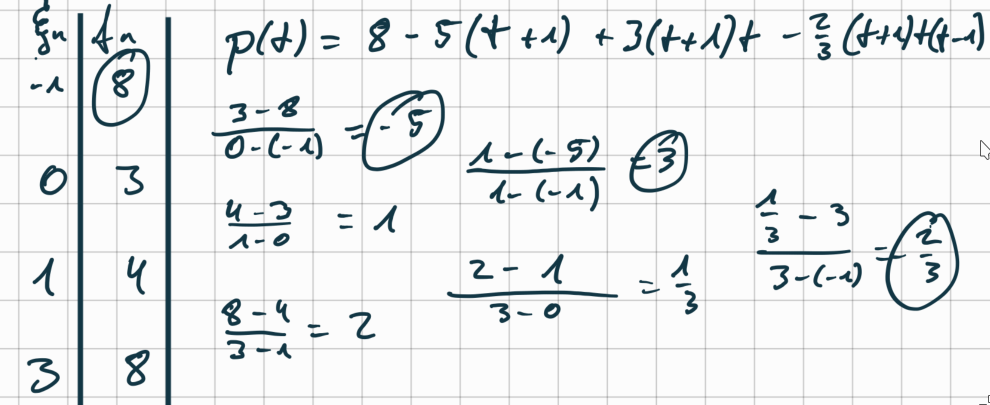
Problem 18: Schema of Neville
Given the table of values:
$$ \begin{array}{|c|c|c|c|c|c|} \hline n & 0 & 1 & 2 & 3 \\ \hline \xi_n & -1 & 0 & 1 & 3 \\ \hline f_n & 8 & 3 & 4 & 8 \\ \hline \end{array} $$a) Determine the interpolation polynomial \(p \in \mathbb{P}_3\) with \(p(\xi_n) = f_n\) for \(n=0, 1, 2, 3\) in Newton form.
b) Extend the interpolation polynomial by including \((\xi_4, f_4) = (2, 1)\).
Solution a)
To calculate the newton poylnomial
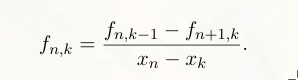
The main diagonal are the coefficients of the newton polynomial.
Solution b)
Problem 19: Fast Cubic Spline
Given the nodes \(\xi_0 = -1, \xi_1 = 0\) and \(\xi_2 = 1\) on the interval \([-1, 1]\). Consider the function
$$ f(t) = \begin{cases} (t+1) + (t+1)^3 & \text{for } -1 \le t \le 0 \\ 4 + (t-1) + (t-1)^3 & \text{for } 0 < t \le 1. \end{cases} $$a) Justify which properties of a cubic spline with natural boundary conditions the function \(f\) fulfills and which it does not.
b) Change the function \(f\) on the subinterval \((0, 1]\) so that \(f\) fulfills all properties of a cubic spline with natural boundary conditions. Hint: The function \(f\) does not need to fulfill any interpolating properties.
Solution a)
First calculate the derivatives
$$ \begin{align*} f_1'(t) &= 1 +3(t+1)^2 \\ f_1''(t) &= 6(t+1) \\ f_2'(t) &= 1+ 3(t-1)^2 \\ f_2''(t) &= 6(t-1) \\ \end{align*} $$Properties
$$ (i) f_1, f_2 \in \mathbb{P}_3 $$$$ (ii) Smoothness: f_1(0) = 2 = f_2(0) f_1'(0) = 4 = f_2'(0) f_1'(0) = 6 \neq -6 = f_2''(0) $$$$ (iii) Natural: f_1''(-1) = 0 f_2''(1) = 0 $$Thus \(f\) fulfills all properties besides continuity in the second derivative in \(t=0\).
Solution b)
For (a) following applies:
$$ \begin{align*} (I) f_2(0) &= 2 \\ (I) f_2'(0) &= 4 \\ (I) f_2''(0) &= 6 \quad f_2''(1) = 0 \end{align*} $$From (III) follows \(f_2''(t) = 6\).
$$ f_2'(t) = -(1-t)^2 + c $$with (II) follows: \(f_2'(0) = -3(1 - 0)^2\).
with (II) follows: \(f_2'(0)\ = -3(1-0)^2 + c =^! u\)
follows \(c=7\), hence \(f_2'(0)\ = -3(1-0)^2 + 7\).
In total we have \(f_2(t) = (1-t)^3 +7t + 1\).
Problem 20: Determining of Weights
Determine the weights \(\omega_0, \omega_1, \omega_2\) for \(\xi_0 = -\frac{h}{2}, \xi_1 = 0\) and \(\xi_2 = \frac{h}{2}\), such that
$$ \int_{-h}^h P(t) \,dt = \sum_{n=0}^2 \omega_n P(\xi_n) $$is exact for polynomials \(P \in \mathbb{P}_2\).
Solution
The basis of \(\mathbb{P}_2\) is \(\{1, x, x^2\}\). Hence the condition of the task is fullfileld when its fullfileld for the basis.
We get the following conditions
$$ \begin{align} \int 1 dt &= [t]^{h}_{-h} = 2h =^{?} \sum w_n 1(\xi_n) = w_0 + w_1 + w_2 \\ \int t dt &= [\frac{1}{2}t^2]^{h}_{-h} = 0 =^{?} \sum w_n t(\xi_n) = -\frac{h}{2} w_0 + \frac{h}{2}w_2\\ \int t^2 dt &= [t]^{h}_{-h} = \frac{2}{3}h^3 =^{?} \sum w_n t^2(\xi_n) = \frac{h^2}{4}w_0 + \frac{h^2}{4}w_2\\ \end{align} $$From (2) follows \(w_0 = w_2\). In (3) we thus get \(\frac{h^2}{2}w_0 = \frac{2}{3}h^3\), from this follows \(w_0 = \frac{4}{3}h = w_2\). In (1) we have \(\frac{8}{3}h + w_2 = 2h\) from this follows \(w_1 = -\frac{2}{3}h\).
Problem 21: Composite (left-sided) rectangle rule
Given is \(f \in C^1[a,b]\), as well as the equidistant nodes for \(n = 0, \dots, N\)
$$\xi_n = a + nh \quad \text{and} \quad h = (b-a)/N.$$The composite (left-sided) rectangle rule is defined by
$$ Q(f) = \sum_{n=1}^N h f(\xi_{n-1}). $$Show the error estimate
$$ \left| \int_a^b f(t) \,dt - Q(f) \right| \leq \frac{b-a}{2} h \sup_{t \in [a,b]} |f'(t)|.$$Solution
From \([\xi_{n-1}, \xi_{n}]\) follows from the taylor series development
$$ f(t) = f(\xi_{n-1})t + f(t_1)f(t - \xi_{n-1}) $$We continue
$$ \begin{align*} \int f(t)dt - Q(f) &= \int_a^b f(t)dt - \sum^N h f(\xi_{n-1}) \\ &= \sum^N (\int_{\xi_{n-1}}^{\xi_n} f(t)dt - h f(\xi_{n-1})) \\ &= \sum^N (\int_{\xi_{n-1}}^{\xi_n} f(\xi_{n-1})t + f(t_1)f(t - \xi_{n-1})dt - hf(\xi_{n-1})) \\ &= \sum^N ([tf(\xi_{n-1})]^{\xi_n}_{\xi_{n-1}} + f(\hat{t}_n) [(t - \xi_{n-1})^2 \cdot \frac{1}{2}]^{\xi_n}_{\xi_{n-1}}) \\ &= \sum^N f'(\hat{t}_n) \frac{1}{2}(\xi_n - \xi_{n-1})^2 \\ &\leq \frac{h}{2} sup |f'(t)| \sum^N \frac{b- a}{N} \\ &= \frac{b-a}{2}h sup |f'(t)| \end{align*} $$Problem 22: Floating Numbers
Given a base \(B \geq 2\), a minimal exponent \(e_{min} \in \mathbb{Z}\) and lengths \(L_m, L_e \in \mathbb{N}\).
(a) Formulate the definition of the set \(FL_+\) of normalized positive floating-point numbers for the given quantities.
(b) Determine \(\max FL_+\) and \(\min FL_+\).
(c) Let \(x \in FL_+\) and let \(y \in FL_+\) be a floating-point number directly adjacent to \(x\). Show that
$$2 \text{ eps } B^{-1} < \frac{|x-y|}{|x|} \leq 2 \text{ eps},$$where eps is the machine epsilon.
(d) State the advantage of choosing \(B = 2\) with regard to the representation of floating-point numbers and formulate estimates analogous to (c), if this advantage is implemented.
Solution a)
$$ FL_+ = \left\{ B^e \sum_{l=1}^{l_m} a_l B^{-l} \;\Bigg|\; e = e_{\min} + \sum_{l=0}^{L_e-1} c_l B^l,\; a_1 \neq 0,\; c_l \in \{0, \dots, B-1\} \right\} $$Solution b)
$$ maxFL_+ = B^{e_{max}} (1- B^{-L_m}) = B^{e_{min} + (B-1) \frac{1 - B^{L_e - 1}}{1 - B}} (1 - B^{-L_m}) = (1 - B^{-L_m})B^{e_{{min} + B^{L_e - 1}}} $$$$ minFL_+ = B^{-1}B^{e_{min}} = B^{e_{min} - 1} $$Solution c)
First
$$ 2 eps B^{-1} = 2 \frac{B^{1-L_m}}{2} B^{-1} = B^{1-L_m}B^{-1} = B^{-L_m} $$Next
$$ 2 eps = \frac{B^{1 - L_m}}{2} = B^{1-L_m} $$And let \(x = mB^e\) than is \(y = (m \pm B^{-L_m})B^e\) thus
$$ \frac{|x -y|}{|x|} = \frac{|mB^e - (m \pm B^{-L_m})B^e|}{mB^e} = \frac{B^{-L_m}}{m} $$With that we have the inequality.
Solution d)
In the case of \(B = 2\) we don’t need to save \(a_1 = 1\). Thus we have an extra bit that we can use for the floating number. Hence the adjucent number \(y = (m \pm B^{-L_m + 1})B^e\).
Then
$$ 2 eps = \frac{B^{1 - L_m+1}}{2} = B^{L_m} = eps $$And
$$ 2 eps B^{-1} = 2 \frac{B^{1-L_m+1}}{2} B^{-1} = B^{1-L_m+1}B^{-1} = B^{-L_m + 1} $$Problem 23: Interpolation Polynomials
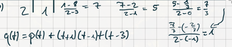
Given the table of values:
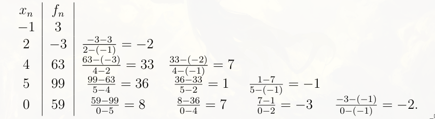
$$ \begin{array}{|c|c|c|c|c|} \hline n & 0 & 1 & 2 & 3 \\ \hline x_n & -1 & 2 & 4 & 5 \\ \hline f_n & 3 & -3 & 63 & 99 \\ \hline \end{array} $$(a) Determine the corresponding interpolation polynomial in Newton form.
(b) We add the point \((x_4, f_4) = (0, 59)\) to the nodes above. Determine the corresponding interpolation polynomial.
(c) Let \(p \in \mathbb{P}_N\) be the interpolation polynomial for a continuous function \(f: [a, b] \to \mathbb{R}\) at the pairwise distinct nodes \(x_0, \dots, x_N \in [a, b]\). Let also \(q \in \mathbb{P}_N\) be arbitrary.
(i) First show that
$$\max_{x \in [a,b]} |q(x) - p(x)| \leq \Lambda_N \max_{x \in [a,b]} |q(x) - f(x)|.$$Give \(\Lambda_N\) explicitly.
(ii) Then show that
$$\max_{x \in [a,b]} |f(x) - p(x)| \leq (1 + \Lambda_N) \max_{x \in [a,b]} |q(x) - f(x)|.$$(iii) Briefly discuss the statement of the estimate in (ii). In doing so, refer to two different classes of nodes from the lecture for \(N \approx 20\).
Solution a)
We have
Thus the newton interpolation polynomial is
$$ p_{0,3}(t) = 3 − 2(t + 1) + 7(t + 1)(t − 2) − (t + 1)(t − 2)(t − 4) $$Solution b)
We have
Thus the newton interpolation polynomial is
$$ p_{0,4}(t) = p_{0,3} 2(t + 1)(t − 2)(t − 4)(t − 5) $$Solution c)
(i) Because p is the polynomial interpolation of f, which means it has the same roots. We have
$$ p(x) = \sum^N p(x_n) L_n(x) = \sum^N f(x_n) L_n(x) $$and
$$ q(x) = \sum^N q(x) L_n(x) $$Hence
$$ \begin{align*} \max |q(x) - p(x)| &= \max |\sum^N q(x_n) L_n(x) - \sum^N f(x_n) L_n(x)| \\ &\leq \max \sum |q(x_n)- f(x_n)| |L_n(x)|\\ &\leq \max \sum |L_n(x)| \max_{x \in x_n} |q(x)- f(x)| \\ &\leq \max \Lambda_N |q(x) - f(x)| \end{align*} $$(ii) We can do
$$ |f (x) − p(x)| = |f (x) − q(x)| + |q(x) − p(x)| $$And now we can use (i)
$$ \max|f (x)−p(x)| \leq \max |f (x)−q(x)| + \max |q(x)−p(x)| \leq (1+Λ N ) \max |f (x)−q(x)|. $$(iii) This formula tells us, how good our interpolation polynomial is, the maximum is \((1 + \Lambda_N)\), where \(\Lambda_N\) is the lebesgue constant.
If we choose aquidistant roots, so is the lebesgue constant very big and the approximation is not useful. For Tschebyscheff roots, the lesbesgue constant is near its minima 1, and we get a useful approximation.
Problem 24: Quadrature Formulas
Let \((b_k, c_k)_{k=1,\dots,s}\) be a quadrature formula of order \(p\).
(a) Formulate the definition of the order as given in the lecture.
(b) Show that if \(p \geq s\), the weights are uniquely determined by the nodes. Give an explicit representation of the weights.
(c) Let \(p \geq s, m \geq 1\) and \(M(x) = (x-c_1) \cdots (x-c_s)\). Show that the order is exactly \(s+m\), if
$$\int_0^1 M(x) g(x) dx = 0$$for all polynomials \(g \in \mathbb{P}_{m-1}\), but not for one of degree \(m\). Hint: Use a representation without proof that could be justified by polynomial division or the Euclidean division algorithm.
(d) Give the maximum order of the quadrature formula. Justify your answer with the help of subproblem (c).
Solution a)
A a quadrature formula \((b_k, c_k)\) has the order \(p\) if for all polynomials from degree \(\leq p-1\) the integral can be calculated exactly, whereby \(p\) is maximal.Solution b)
The lagrange Polynomial \(L_n\) are determinted through the knots \(c_1, .., c_s\). For the order \(p \geq s\), follows with \(L_j(c_k) = \delta_{jk}\)
$$ \int_0^1 L_j(x) dx = \sum^s b_k L_j(ck) = b_j $$Solution c)
Let \(f \in \mathbb{P}_{s + m - 1}\) be arbitrarily. Then exist a polynomial \(g \in \mathbb{P}_{m-1}\) and \(r \in \mathbb{P}_{s-1}\) with \(f = Mg + r\) because of polynomial division.
And
$$ \int f(x) dx = \int M(g)g(x) fx + \int r(x) dx $$and the same for their interpolation
$$ \sum b_k f(c_k) = \sum b_k M(c_k)g(c_k) + \sum b_k r_k(c_k) $$And because \(p \geq s\) the last summands of both formulas are the same. Hence the polynomial inteprolcation calculates the exact integral.
From this follows that the order is exactly then \(m +s\) when
$$ \int M(x)g(x) dx = 0 $$for all polynomials of order \(\leq m-1\), but not for ones of order \(m\).
Solution d)
The maximum order we can have is \(2s\) because that would mean that we have \(g = M\) and then
$$ \int M(x)g(x) dx = \int M(x)^2 dx > 0 $$Problem 25: Matrices
Let \(A, B \in \mathbb{R}^{N \times N}\) and \(\|\cdot\|\) be an arbitrary norm on \(\mathbb{R}^N\).
(a) For the corresponding matrix norm, show the submultiplicativity \(\|AB\| \leq \|A\| \|B\|\).
(b) Let \(A\) be regular. Show that \(\text{cond}(A) \geq 1\).
(c) Let \(A\) be regular, \(\mathbf{b}, \tilde{\mathbf{b}} \in \mathbb{R}^N\) and \(\mathbf{x}, \tilde{\mathbf{x}} \in \mathbb{R}^N\) with \(A\mathbf{x} = \mathbf{b}\) and \(A\tilde{\mathbf{x}} = \tilde{\mathbf{b}}\). Show that
$$\frac{\|\mathbf{x} - \tilde{\mathbf{x}}\|}{\|\mathbf{x}\|} \leq \text{cond}(A) \frac{\|\mathbf{b} - \tilde{\mathbf{b}}\|}{\|\mathbf{b}\|}$$and briefly discuss the estimate.
(d) Let \(\mathbf{v} \in \mathbb{R}^N\) be arbitrary and let \(\mathbf{e} \in \mathbb{R}^N\) be the vector consisting of all ones. Determine the spectrum of \(\mathbf{e}\mathbf{e}^T\) and the value \(\|\mathbf{v}\mathbf{e}^T\|_2\).
Solution a)
We have \(||A|| = \sup \frac{||Ax||}{||x||} = \max ||Ax||\). Hence
$$ ||AB|| = \max ||ABx|| \leq \max ||A|| ||Bx|| = ||A|| \max ||Bx|| = ||A||||B|| $$Solution b)
We have
$$ 1 = ||I_n|| = ||A^{-1}A|| \leq ||A^{-1}||||A|| = cond(A) $$Solution c)
Because \(Ax=b\) we can rwrite
$$ x - \hat{x} = A^{-1}b - A^{-1}\hat{b} $$Thus
$$ ||x- \hat{x}|| = ||A^{-1}(b - \hat{b})|| \leq ||A^{-1}||||b - \hat{b}|| $$And with that
$$ \frac{||x - \hat{x}||}{||x||} \leq \frac{||A^{-1}||||b - \hat{b}||}{||x||} = \frac{||b||||A^{-1}||||b - \hat{b}||}{||x||||b||} = \frac{||b||||A^{-1}||}{||x||}\frac{||b - \hat{b}||}{||b||} \leq ||A||||A^{-1}|| \frac{||b - \hat{b}||}{||b||} $$For this approximation to be useful the error of \(\frac{||b - \hat{b}||}{||b||}\) needs to be small.
If our condition number is small this approximation guarantees, that small errors in \(b\) lead to small innacuracies from \(x\). Is the condition number nig, so can even a small error lead to a big error in our solution, but it doesnt have to be, because the right side of the approximation is so loose.
Solution d)
Because \(e \neq 0\), is \(ee^T\) a Matrix with rang 1. Hence 0 is a eigenvalue with the multiplicity of \(N-1\).
Next, \(Kern(ee^T) = span\{e\}^T\).
In addition we have the eigenvalue \(N > 0\) because \(ee^Te = e^Tee = Ne\). With that we have the spectrum.
Next with \(ev^Tve^T = ||v||_2^2ee^T\) we get
$$ ||ve^T||_2 = \sqrt{\max{\lambda \in ev^Tve^T}} = ||v||_2 \sqrt{\max{\lambda \in ee^T}} = ||v||_2 \sqrt{N} $$Problem 26: CG-Algorithm
Let \(A\) be a symmetrical positive definite matrix and \(x^*\) be the solution of the LGS \(Ax = b\).
What is the function \(\phi\), that the CG_Algorithm minimizes? What is the connection to the LGS \(Ax =b\)?
Solution
We have \(\phi(x) = \frac{1}{2}x^TAx - x^Tb\), which gets minimized by the CG-Algorithm.
A necessary condition for the minima \(x^*\) is that \(\phi(x^*) = (Ax^* -b)^T = 0^T\). This condition is because of \(\phi''(x) = A\) symmetrical and positive definite also sufficient.
Hence is \(x^*\) then the minima from \(\phi\), if \(x^*\) solves the LGS \(Ax = b\).
Problem 27: LR- and Cholesky-Decomposition
(a) Solve \(Ly = b\) by forward substitution for
$$L = \begin{pmatrix} 2 & 0 & 0 \\ -2 & -1 & 0 \\ 3 & 2 & 1 \end{pmatrix}, \quad b = \begin{pmatrix} 4 \\ -3 \\ 6 \end{pmatrix}.$$(b) State the conditions on a matrix \(A \in \mathbb{R}^{N \times N}\) under which a Cholesky decomposition exists, and in the case \(N=3\), derive three formulas for the entries of the Cholesky factor \(L \in \mathbb{R}^{3 \times 3}\) of such a matrix. It is not necessary to express all coefficients of \(L\) solely in terms of coefficients of \(A\), as long as you consider the order of the calculations.
(c) Let \(A \in \mathbb{R}^{M \times N}\), \(M \geq N\) and \(b \in \mathbb{R}^M\). (i) Give the normal equation for the least squares problem \(\min_{x \in \mathbb{R}^N} \|Ax - b\|_2^2\).
(ii) Name an additional condition on \(A\) such that the normal equation could be solved by a Cholesky decomposition, and determine the effort (with respect to \(M\) and \(N\)) of the Cholesky decomposition for the normal equation.
(iii) Name an iterative method to solve the normal equation under the condition from (ii) and determine the main effort of one step of the method for the normal equation (with respect to \(M\) and \(N\)).
Solution a)
We have
$$ \begin{align*} 2y_1 = 4 &\implies y_1 = 2 \\ -2 \cdot 2 -y_2 = -3 &\implies y_2 = -1 \\ 3 \cdot 2 + 2 \cdot (-1) + 1 y_3 = 6 &\implies y_3 =2 \end{align*} $$Hence
$$ y = (2 \ -1 \ 2)^T $$Solution b)
A choleky decomposition exists if and only if, the matrix symmetrical and positive definite(spd).
$$ \begin{pmatrix} a_{11} & a_{12} & a_{13} \\ a_{21} & a_{22} & a_{23} \\ a_{31} & a_{32} & a_{33} \end{pmatrix} = \begin{pmatrix} l_{11} & 0 & 0 \\ l_{21} & l_{22} & 0 \\ l_{31} & l_{32} & l_{33} \end{pmatrix} \cdot \begin{pmatrix} l_{11} & l_{21} & l_{31} \\ 0 & l_{22} & l_{32} \\ 0 & 0 & l_{33} \end{pmatrix} = \begin{pmatrix} l_{11}^2 & l_{21}l_{11} & l_{31}l_{11} \\ l_{21}l_{11} & l_{22}^2 + l_{21}^2 & l_{21}l_{31} + l_{22}l_{32} \\ l_{31}l_{11} & l_{21}l_{31} + l_{22}l_{32} & l_{33}^2 + l_{32}^2 + l_{31}^2 \end{pmatrix} $$Hence
$$ \begin{align*} l_{11} &= \sqrt{a_{11}} \\ l_{21} &= a_{21}/\sqrt{a_{11}} \\ l_{31} &= a_{31}/\sqrt{a_{11}} \\ &... \end{align*} $$Solution c)
(i) \(A^TAx = A^Tb\)
(ii) Is the rang of \(A\) maximal so is \(A^TA\) symmetrical and positive definite and can thus be solves using the cholesky decomposition.
The cholesky deocmpositon needs \(1/2 MN^2\) operation, but because \(N=M\) and it is symmetrcial, we need \(1/6 N^3\) operations.
(iii) Another algorithm we can use to solve the normal equation is the CG-Algorithm. We need to do 2 matrix-vector products, as such we need to do \(2NM\) operations.
Problem 28: CG-Algorithm
Complete the following content (a) to (i).
The cg-method is used to solve linear systems of equations of the form \(Ax=b\) with \(A \in \mathbb{R}^{N \times N}\). The necessary conditions for the matrix \(A\) to be able to apply the cg-method are \((a)\) . Instead of solving the linear system directly, the following functional \(\Phi(x) = \) \((b)\) is minimized. The main idea is to solve iteratively one-dimensional minimization problems: Let \(x^k \in \mathbb{R}^N\) and the \((c)\)______ \(d^k \in \mathbb{R}^N \setminus \{0\}\) be given, then \(\alpha_k\) is calculated such that \(\varphi(\alpha) = \Phi(x^k + \alpha d^k)\) is minimal. A sufficient condition for the determination of \(\alpha_k\) is \((d)\). The new approximation \(x^{k+1}\) is then calculated by \((e)\). Theoretically, the cg-method provides the exact solution after \((f)\)______ steps. The main effort of the cg-method lies in the calculation of \((g)\). By \((h)\) the number of steps and thus the total effort can be reduced. The cg-method is particularly well suited for very large and/or \((i)\)______ matrices.
Solution
(a) symmetrical and positive definite
(b) \( \phi = 1/2x^Txx^Tb \)
(c) Search direction
(d) (\phi’(\alpha_k) = 0)
(e) \(x^{k+1} = x^k + \alpha_kd^k\)
(f) N
(g) \(Ad^k\) the matrix vector product
(h) Preconditioning
(i) sparse
Problem 29: Machine accuracy
Explain the course of the graph in the plot, which was generated by evaluating the function \(\frac{(1+x)-1}{x}\) for \(0 < x \leq 10^{-15}\) with a machine precision of \(\text{eps} \approx 2.2 \cdot 10^{-16}\), by giving the exact reasoning:
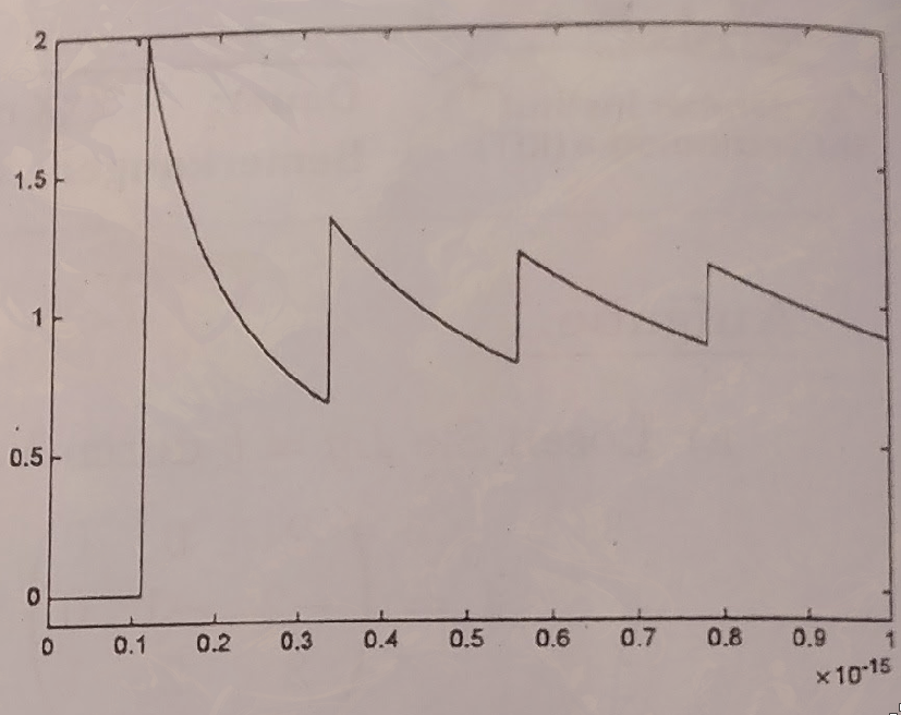
(a) for the constant value equal to 0 at the far left of the graph,
(b) for the first jump of the graph from 0 to 2,
(c) and for the behavior of the function between the first two jumps.
(d) Additionally, state the function values at the second jump. Justify briefly.
Solution a)
The graph goes until \(1.1 \cdot 10^{-16}\) which is exactly \(eps/2\), as such we round down from \(1 +x\) to \(1\) as such we have \(0/x = 0\).Solution b)
After \(1.1 \cdot 10^{-16}\) we are above \(eps/2\) as such we round up, from \(1 + x\) to \(1 + eps\). Hence \(1 + eps -1/eps/2 = eps/eps/2 = 2\).Solution c)
The next section in the graph is between \(eps/2\) and \(3eps/2\), in this section \(1 + x\) is constant and bigger than zero.Solution d)
When we reach \(3eps/2\) we have the same effect as in (a), but instead we get \(eps/3/2eps = 2/3\).Problem 30: QR-Decomposition
Given a QR decomposition of the matrix \(A\).
$$ Q = \frac{1}{15} \begin{pmatrix} 5 & -2 & -14 \\ 10 & 11 & 2 \\ 10 & -10 & 5 \end{pmatrix}, \quad R = \begin{pmatrix} 3 & 1 \\ 0 & -5 \\ 0 & 0 \end{pmatrix}, \quad A = \begin{pmatrix} 1 & 1 \\ 2 & -3 \\ 2 & 4 \end{pmatrix}0 .$$It holds that \(A=QR\), where you can use the fact that \(Q\) is an orthogonal matrix.
(a) Using the given decomposition, explain which of the overdetermined systems \(Ax=b\) and \(Ax=\tilde{b}\) are solvable, where
$$(i) \quad b = \begin{pmatrix} 0 \\ -5 \\ 2 \end{pmatrix}, \quad (ii) \quad \tilde{b} = \begin{pmatrix} 0 \\ -5 \\ 4 \end{pmatrix}. $$(b) In both cases, use the QR decomposition to calculate the solutions to the corresponding least squares problems.
(c) Calculate the residuals for these solutions.
Solution a)
We have \(Ax = b \iff QRx = b \iff Rx = Q^Tb\).
(i)
$$ Q^Tb = \frac{1}{15} \begin{pmatrix} 5 & -2 & -14 \\ 10 & 11 & 2 \\ 10 & -10 & 5 \end{pmatrix} \begin{pmatrix} 0 \\ -5 \\ 2 \end{pmatrix} = \frac{1}{15} \begin{pmatrix} -30 \\ -75 \\ 0 \end{pmatrix} = \begin{pmatrix} -2 \\ -5 \\ 0 \end{pmatrix} $$Thus we have the LGS
$$ \left( \begin{array}{cc|c} 3 & 1 & -2 \\ 0 & -5 & -5 \\ 0 & 0 & 0 \end{array} \right) $$which has a solution with \(x=(-1 \ 1 )^T\).
(ii)
$$ Q^T\tilde{b} = \frac{1}{15} \begin{pmatrix} 5 & -2 & -14 \\ 10 & 11 & 2 \\ 10 & -10 & 5 \end{pmatrix} \begin{pmatrix} 0 \\ -5 \\ 4 \end{pmatrix} = \frac{1}{15} \begin{pmatrix} -10 \\ -95 \\ 10 \end{pmatrix} = \frac{1}{3} \begin{pmatrix} -2 \\ -19 \\ 0 \end{pmatrix} $$This is not solvable because the last entry is not \(0\), and in the LGS we have has a \(0\) there.
Solution b)
See (a) for \(b\) the solution is \(x = (-1, 1)^T\).
For \(\tilde{b}\), the LGS might not be solvable but we can solve the corresponding least square problem. For that we solve
$$ \left( \begin{array}{cc|c} 3 & 1 & -2/3 \\ 0 & -5 & -19/3 \\ 0 & 0 & 0 \end{array} \right) $$which is \(x^* = (-29/45, \ 19/15)^T\).
Solution c)
The residium for \(b\) is \(Ax -b = Q(Rx - Q^Tb) = 0\)
The residium for \(\tilde{b}\) is
$$ Ax - \tilde{b} = Q(R\tilde{x} - Q^T)\tilde{b} = \frac{2}{9} (2 \ -2 \ 1)^T $$Problem 31: Splines
(a) Let nodes \(a = x_0 < \dots < x_N = b\) and corresponding values \(y_0, \dots, y_N \in \mathbb{R}\) be given. Give the definition of a natural interpolating cubic spline for \((x_0, y_0), \dots, (x_N, y_N)\).
(b) Determine \(\alpha, \beta, \gamma \in \mathbb{R}\) such that the function \(s: [0, 2] \to \mathbb{R}\) defined by
$$s(x) = \begin{cases} -x^3 + 8x + \alpha, & 0 \leq x \leq 1, \\ \beta x^3 + \gamma x^2 + 14x - 1, & 1 < x \leq 2 \end{cases}$$is a cubic spline for \(x_0=0, x_1=1\) and \(x_2=2\).
(c) Decide whether this spline is a periodic spline. Justify your answer briefly.
Solution a)
A natural interpolation cubic splines fulfills the following conditions:
$$ \begin{align*} &(i) s{[x_n, x_{n+1}]} \in \mathbb{P}_3\\\ &(ii) s \in C^2[0,2]\\ &(iii) s(x_n) = y_n \forall x \in \{0,...,N-1\}\\ &(iv) s''(x_0) = s''(x_N) = 0 \end{align*} $$Solution b)
We first calculate the derivatives
$$ S'(x) = \begin{cases} -3x^2 + 8 \\ 3\beta x^2 + \gamma x + 14 \end{cases} $$and
$$ S''(x) = \begin{cases} -6x \\ 6\beta x + \gamma \end{cases} $$We get the conditions
$$ \begin{align*} S_{[0,1]}(1) &= S_{[1,2]}(1) \\ S'_{[0,1]}(1) &= S'_{[1,2]}(1) \\ S''_{[0,1]}(1) &= S''_{[1,2]}(1) \\ \end{align*} $$Hence
$$ \begin{align*} 7+ \alpha &= \beta + \gamma + 13 \\ 5 &= 3\beta + 2 \gamma + 14 \\ -6 &= 6 \beta + 2\gamma \end{align*} $$From this we get the LGS
$$ \left( \begin{array}{ccc|c} 1 & -1 & -1 & 6 \\ 0 & -3 & -2 & 9 \\ 0 & 6 & 2 & -6 \end{array} \right) $$The solution of it, is \(\alpha=1, \beta=1, \gamma=-6\).
Solution c)
A spline is periodic if and only if \(s'(a) = s'(b) \land s''(a) = s''(b)\) is fulfilled.
$$ S(0) = 1 \neq 11 = S(2) $$Problem 32: Quadraturformula
(a) Let a quadrature formula with nodes \(c_k\) and weights \(b_k\), for \(k=1, \dots, s\), be given. (i) Give the definition of the order \(p\) of a quadrature formula. (ii) Name the order conditions for a quadrature formula of order 2. (iii) Give the order that a quadrature formula with \(s\) nodes can have at most.
(b) How many nodes are necessary for polynomial interpolation to uniquely determine a polynomial of degree \(N\)? Briefly justify why this interpolation polynomial is unique.
(c) Give the formula for the nodes of Chebyshev interpolation on the interval \([-1, 1]\). Briefly explain what advantages this choice offers over an equidistant one.
(d) Let \(p\) be a polynomial of degree \(N \ge 1\) in \(\mathbb{R}^d\). State how the graph \(\Gamma_p\) of \(p\) can be interpreted as a polynomial of degree \(N\) in \(\mathbb{R}^{d+1}\), and explain what the control points of \(p\) are.
(e) A point of intersection of the circle \(x^2 + y^2 = 2\) and the hyperbola \(x^2 - y^2 = 1\) is to be calculated numerically. (i) Give the formulation of the problem so that the Newton method can be applied to it. (ii) Calculate the first iterate for this problem with a starting value of \((1, -1)^T\).
Solution a)
(i) A quadrature formula has exactly order \(p\) if and only if the integral of the interpolation polynomial is exactly the solution for all polynomials with degree less than \(p-1\), whereby \(p\) is the maximum.
(ii) The general quadratur formula order condition is
$$ \frac{1}{q} = \sum_{k=1}^s b_k c_k^{q-1} $$a formula has the order p if this condition is fulfilled for p but not for \(q = p +1\).
This means we have the following two coniditons
$$ \begin{align*} 1 &= \sum^s b_k \\ 1/2 &= \sum^s b_kc_k \\ 1/3 &\neq \sum b_k c_k^2 \end{align*} $$(iii) The maximum is \(2s\), because then \(\int M(x)g(x) = \int M(x)^2 \neq 0\).
Solution b)
To determine a polynomial of degree \(N\) exactly we need \(N+1\) roots, because of the fundamental lemma of algebra. If we had two different polynomials \(p,q\), then \(p-q\) has \(N+1\) roots and the polynomial degree \(N\), but this is only true for the zero polynomial, hence the polynomials need to be the same, Contradiction. Thus we have only one polynomial.Solution c)
The roots are
$$ x_n = \cos(\frac{2n + 1}{2N +2}\pi) $$The advantage is we have fewer oscillations and the condition is better in comparison to equidistant roots.
Solution d)
$$ \Gamma_p(x) = (0 \ v_0)^T + (1 \ v_1)^Tx + ... + (0 \ v_n)x^N $$The control points are the coefficients of \(p\) of the berstein polynomial \(p(x) = \sum_{n=0}^{N} b_n B_n^N(x)\).
Solution e)
(i) The newton method solves zero point problems, thus \(F(x, y) := (x^2 + y^2 - 2, x^2 - y² -1)^T = 0\)
(ii) To calculate the first iteration \(x^1 = x^0 + \delta x\) we need to solve the LGS
$$ \delta x = -F'(1, -1)^{-1}F(-1, 1)^T $$The Jacobi Matrix of this is
$$ F'(x,y)= \begin{pmatrix} 2x & 2y \\ 2x & -2y \end{pmatrix} $$We need to check this at the point \(x_0\)
$$ F'(1,-1)= \begin{pmatrix} 2 & -2 \\ 2 & 2 \end{pmatrix} $$Thus
$$ \delta x = \frac{1}{4} \begin{pmatrix} 1 & 1 \\ -1 & 1 \end{pmatrix} \begin{pmatrix} 0 \\ -1 \end{pmatrix} = \frac{1}{4} \begin{pmatrix} 1 \\ -1 \end{pmatrix} $$Hence
$$ x^1 = (\frac{5}{4}, - \frac{3}{4}) $$Problem 33: LR and QR-decomposition
Given the linear system of equations \(Mx = \mathbf{b}\) with a regular matrix
$$ M = \begin{pmatrix} A & B \\ 0 & C \end{pmatrix} \in \mathbb{R}^{(N+K)\times(N+K)}, \quad \mathbf{b} = \begin{pmatrix} \mathbf{b}^1 \\ \mathbf{b}^2 \end{pmatrix} \in \mathbb{R}^{N+K}, $$where \(A \in \mathbb{R}^{N \times N}, B \in \mathbb{R}^{N \times K}, C \in \mathbb{R}^{K \times K}, \mathbf{b}^1 \in \mathbb{R}^N\) and \(\mathbf{b}^2 \in \mathbb{R}^K\).
An \(LR\)-decomposition \(PA = LR_A\) of \(A\) and a \(QR\)-decomposition \(C = QR_C\) of \(C\) are already known. The matrices \(A\), \(B\), and \(C\) are assumed to be full.
(a) State how many operations were necessary for the computation of the \(LR\)- and \(QR\)-decompositions, respectively.
(b) Explain how you can efficiently solve the system of equations \(Mx = \mathbf{b}\) using these two decompositions.
(c) Determine the computational cost for solving \(Mx = \mathbf{b}\) without the decompositions, by stating the cost for each sub-step.
(d) Explain the procedure for the linear system of equations \(M^T\mathbf{x} = \mathbf{b}\) by cleverly using both decompositions. The computational cost is not requested here.
Solution a)
For LR-Decomposition we need \(1/3 N^3\) operation. For QR-Decomposition we need \(2/3MN^2=2/3K^3\) operation.Solution b)
This means
$$ Ax_1 + Bx_2 = b_1 \iff Ax_1 = b_1 - Bx_2 $$and
$$ Cx_2 = b_2 $$Hence
- Solve \(Q c = b_2 \iff c = Q^Tb_2\)
- Solve \(R x_2 = c\) using backward substitution
- Solve \(Rc = P(b_a - Bx_2)\) forward substitution
- Solve \(L x_1 = c\) backwards substitution
Solution c)
- \(K^2\) operations
- \(1/2 K^2\) operations
- \(0 + N+NK\) operations
- \(1/2N^2\) operations
Solution d)
We now have
$$ M^T = \begin{pmatrix} A^T & 0 \\ B^T & C^T \end{pmatrix} $$Hence
$$ (i) \quad Ax_1 = b_1 $$and
$$ (ii) \quad Bx_1 + Cx_2 = b_2 \iff Cx_2 = b_2 - Bx_1 $$We can solve it using
$$ PA = LR \iff A^T = R_A^TL^T $$and
$$ C = QR \iff C^T = R_c^TQ^T $$Then solve (i) using the first decomposition and (ii) using the second decompsotion.
Problem 34: Newton Method and Floating Numbers
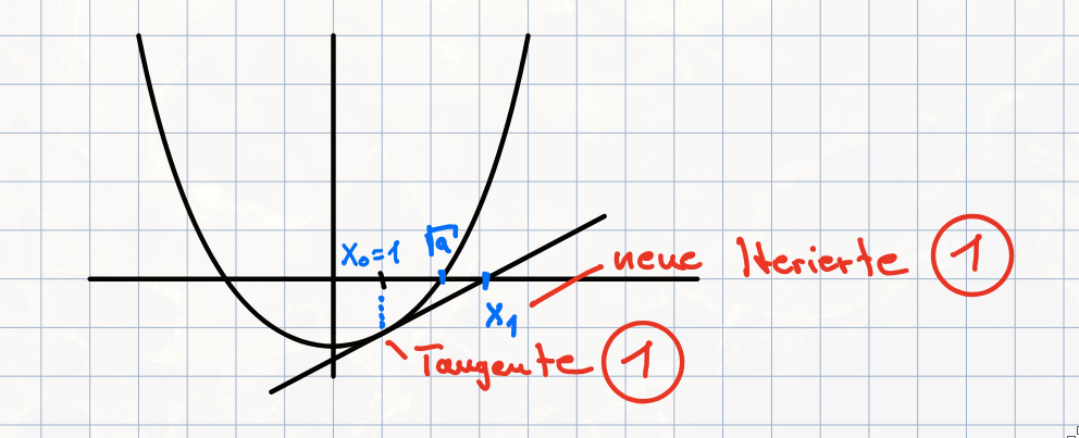
The goal is to approximate \(\sqrt{a}\) for \(a > 1\).
(a) State the function \(f: \mathbb{R} \to \mathbb{R}\) proposed in the lecture and the corresponding Newton’s method to approximately determine \(\sqrt{a}\).
(b) Create a sketch and illustrate in it that with the starting value \(x_0 = 1\), it follows that \(x_1 > \sqrt{a}\), where \(x_1\) denotes the first Newton iterate.
(c) Use the concrete representation of floating-point numbers in the IEEE Double-Precision standard to justify that one must ultimately only be able to calculate square roots of numbers from the interval \((1, 4)\).
(d) We want to use a computer in the IEEE Double-Precision standard to calculate the expression \(\sqrt{x^2 + y^2}\) for \(x = \mathrm{fl}(\pi \cdot 10^{160})\) and \(y = \mathrm{fl}(e \cdot 10^{150})\). Explain which problem will arise with a naive calculation and how the problem can be remedied. Additionally, determine the value that the computer calculates with the remedied variant.
Hint: \(\sqrt{x^2 + y^2} = \sqrt{x^2(1 + \frac{y^2}{x^2})} = |x|\sqrt{1 + \frac{y^2}{x^2}}\) might be helpful.
Solution a)
The newton-method works as follows:
$$ x^{k+1} = x^k + d^k $$with
$$ f'(x)d^k = -f(x) $$we repeat this until \(||d^k|| < \epsilon\).
And where \(f(x) = x^2 - a\) and \(f'(x)=x\)
Solution b)
Solution c)
In IEEE we have \(a = (1+m)2^e\) with \(0 \leq m \le 1\).
If \(e\) is even, then \(a = (1+m)2^2k\), hence \(\sqrt{a} = \sqrt{(1+m)}2^k\), where \(m' \in (1, 2)\)
If \(e\) is uneven, then \(a = (1+m)2^{2k+1}\), hence \(\sqrt{a} = \sqrt{(1+m)}2^{(2k+1)/2} = \sqrt{2(2+m)}2^{(2k)/2}\) where \(m' \in (2,4)\)
Solution d)
Because of \(x^2 = \pi^2 \cdot 10^{320} > 10^{308}\) we have an overflow.
We can use the hint and \(\sqrt{x^2 +y^2} = x \sqrt{1 + \frac{y}{x}}^2\). Here we have no overflow, because
$$ 0 \le (y/x)^2 \le e^2/\pi^2 10^{-20} \le eps/2 $$Problem 35: Matrices and Norms
(a) Prove \(\|A\|_{\infty} = \max_{n=1,\dots,N} \sum_{m=1}^N |a_{nm}|\) for \(A \in \mathbb{R}^{N \times N}\).
(b) Show that \(\mathrm{cond}_2(Q) = 1\) for every orthogonal matrix \(Q \in \mathbb{R}^{N \times N}\).
(c) Let \(\mathbf{e} \in \mathbb{R}^N\) be the vector consisting of all ones. Show that \(\|\mathbf{v}\mathbf{e}^\top\|_1 = \|\mathbf{v}\|_1\) for every vector \(\mathbf{v} \in \mathbb{R}^N\).
(d) Let \(A \in \mathbb{R}^{N \times N}\) be regular, \(\|\cdot\|\) a norm on \(\mathbb{R}^N\) with the corresponding induced matrix norm \(\|\cdot\|\), and \(\mathbf{x} \in \mathbb{R}^N\). Let \(\tilde{\mathbf{x}}\) be a perturbation of \(\mathbf{x}\). Derive an upper bound for the relative error of the product \(A\mathbf{x}\) as a function of the relative perturbation in \(\mathbf{x}\) (\(A\) remains unperturbed), by proving and then using \(\|\mathbf{x}\| \le \|A^{-1}\| \|A\mathbf{x}\|\).
Solution a)
$$ ||A||_\infty = \max_{||x|| = 1} ||Ax||_{\infty} $$Further
$$ ||Ax||_{\infty} = \max_{n=1,...,N} |\sum a_{nm}x_m| \leq \max_{n=1,...,N} \sum |a_{nm}| |x_m| $$where \(||x_m||_\infty = 1\).
Solution b)
We have
$$ ||Q||_2 = \max_{||x||_2 = 1} ||Qx||_2 = 1 $$Hence
$$ cond_2(Q) = ||Q||_2 ||Q^T||_2 = ||Q||_2^2 = 1 $$Solution c)
$$ ||ve^T||_1 = max \sum |a_nm| = \sum |v_n| = ||v||_1 $$Problem 36: Quadrature formulas
Let a quadrature formula \((b_k, c_k)_{k=1,\ldots,s}\) be given.
(a) Formulate the definition of the order \(p\) of a quadrature formula.
(b) Give the Lagrange polynomial \(L_j\) for the nodes \(c_1 < \dots < c_s\).
Hint: \(f\) is called point-symmetric if \(f(-x) = -f(x)\) for \(x \in [-1, 1]\).
(c) Give a symmetric quadrature formula of your choice.
Solution a)
A quadraturformel has the order \(p\) then, when it can exactly integrate for all polynomial with degree \(\leq p-1\) and where \(p\) is maximal.Solution b)
$$ L_j = \prod \frac{x - c_k}{c_j - c_k} $$Solution c)
Trapezrule \((a-b)(f(a)-f(b))/2\).Problem 37: Short Questions
(a) Given are the points \((t_n, y_n)\), \(n = 1, 2, 3, 4\), with
$$\begin{array}{c|cccc} t_n & 0 & 1 & 2 & 3 \\ \hline y_n & -2 & -1 & 0 & 2 \end{array}.$$A quadratic function \(g(t) = \alpha + \beta t + \gamma t^2\), \(\alpha, \beta, \gamma \in \mathbb{R}\), is sought, such that \(\sum_{n=1}^4 |g(t_n) - y_n|^2\) is minimized. Formulate the corresponding linear least squares problem and give the general form of the corresponding normal equations.
(b) Determine the Householder transformation \(Q\) that is free from cancellation errors, such that \(QAQ = \begin{pmatrix} * & * & * \\ * & * & * \\ 0 & * & * \end{pmatrix}\) holds for
$$A = \begin{pmatrix} 1 & -1 & 2 \\ 3 & 0 & 1 \\ 4 & 1 & 0 \end{pmatrix}.$$Briefly explain why the \(*\)-structure is achieved this way.
(c) Let \(s: [a, b] \to \mathbb{R}\) be a cubic interpolating spline for the support points \((x_n, y_n)\), \(n = 0, \ldots, N\), with \(s'(a) = s'(b) = 0\). Formulate the definition of the Lagrange splines \(l_n\) for \(n = 0, \ldots, N\) and represent \(s\) using these.
(d) Give a class of matrices for which the singular values correspond to the eigenvalues. Justify your answer briefly.
Solution a)
Linear least square problem:
$$ min ||A(\alpha \ \ \beta \ \ \gamma)^T - b||_2 $$with
$$ b = (-2 \ \ -1 \ \ 0 \ \ 2)^T $$and
$$ A = \begin{pmatrix} 1 & 0 & 0 \\ 1 & 1 & 1 \\ 1 & 2 & 4 \\ 1 & 3 & 9 \end{pmatrix} $$Normal equations:
$$ A^TAx = A^Tb $$Solution b)
We do a householder transformation
$$ \hat{Q} = I_2 - 2\hat{w}\hat{w}^T $$and
$$ \hat{w} = (3 \ \ 4)^T + 5 (1 \ \ 0)^T/||(8 \ \ 4)||_2 = 1/\sqrt{80}(8 \ \ 4)^T $$With \(w = (0 \ \ \hat{w})\) and
$$ Q = I_3 - ww^T = \begin{pmatrix} 1 & 0 \\ 0 & \hat{Q} \end{pmatrix} $$And because \(Qe^1 = e^1\) we have \(QAQ\) as in the task.
Solution c)
\(l_n\) is a cubic interpolation spline with the roots \((x_n, y_n)\) with \(l_n'(a) = l_n(b) = 0\).
And: \(s_n(x) = \sum y_n l_n(x_)\)
Solution d)
The identity matrix because its eigenvaleus are 1 and the square root of 1 is 1.
Better Alternative: All spd Matrices, because \(\lambda\) EV from A \(\iff\) \(\lambda^2\) EV from \(A^TA\) \(\iff\) \(\lambda = \sqrt{\lambda^2}\) Singular value from \(A\).
Problem 38: Cholesky
Let \(A \in \mathbb{R}^{N \times N}\) be a symmetric positive definite matrix.
(a) Explain how and with what computational cost \(\det(A)\) can be calculated efficiently.
For given vectors \(\mathbf{u}, \mathbf{v}, \mathbf{b} \in \mathbb{R}^N\) and \(d, c \in \mathbb{R}\), we now consider the linear system of equations (sought are \(\mathbf{x} \in \mathbb{R}^N\) and \(y \in \mathbb{R}\))
$$\begin{pmatrix} A & \mathbf{u} \\ \mathbf{v}^\top & d \end{pmatrix} \begin{pmatrix} \mathbf{x} \\ y \end{pmatrix} = \begin{pmatrix} \mathbf{b} \\ c \end{pmatrix} \quad (1)$$with unknown solution \(\mathbf{x}^* \in \mathbb{R}^N\) and \(y^* \in \mathbb{R}\), where a Cholesky decomposition of matrix \(A\) is known.
(b) First, derive an explicit formula for \(y^*\) independent of \(\mathbf{x}^*\) under the assumption \(d - \mathbf{v}^\top A^{-1} \mathbf{u} \neq 0\).
(c) Explain how and with what computational cost \(y^*\) can be calculated numerically efficiently.
(d) Investigate under what conditions the matrix in (1) is symmetric and positive definite, using the Cholesky decomposition of \(A\).
Solution a)
Since the matrix is spd we can do a cholesky decomposition in \(A = LL^T\) with \(det(A) = det(L)det(L^T)\) cholesky takes \(1/6N^2\) operations and we can calculate the determinant by \(\prod l_{nn}\).Solution b)
We have
$$ Ax + uy = b \iff x = A^{-1}(b - uy) $$and
$$ v^Tx + dy = c \iff v^TA^{-1}b - v^TA^{-1}uy + dy = c $$Hence
$$ y = \frac{c - v^TA^{-1}b}{d - v^TA^{-1}u} $$Solution c)
The expensive part to calculate is \(v^TA^{-1}\), we thus want to calculate this efficiently by using the cholesky decomposition. For this we define \(\hat{v} = v^TA^{-1}\) then \(v^TA^{-1} = v^TA^{-1} \iff A^Tv^TA^{-1} = v \iff A^T\hat{v} = v\). Then we can solve as follows
- \(L^ \hat{\hat{v}} = v\) forward substitution
- \(L^T \hat{v} = \hat{\hat{v}}\) backward substitution
- Calculate Scalarproduct of \(\hat{v}^Tb\) and \(\hat{v}^Tu\)
This takes in total \(N^2 + 2N\) operations.
Solution d)
Symmetry:
$$ \begin{pmatrix} A & \mathbf{u} \\ \mathbf{v}^\top & d \end{pmatrix}^T = \begin{pmatrix} A^T & \mathbf{v} \\ \mathbf{u}^T & d \end{pmatrix} $$This means the matrix is then symmetrical if \(v = u\).
Positive definite:
The matrix is exactly then positive definite if a cholesky decomposition exists.
Problem 39: Interpolation polynomial
(a) Let the support points \((x_0, f_0), \ldots, (x_N, f_N)\) be given. Formulate the definition of the interpolation polynomial and prove that such a polynomial exists.
(b) Determine the interpolation polynomial in Newton form for the support points \((1, 16)\), \((3, 4)\) and \((5, 8)\), explicitly stating the Newton polynomials.
Solution a)
Let \(p\) be the interpolation polynomial then the following needs to apply:
- \(p_{|x_{n-1};x_{n}} \in P\)
- \(p(x_n) = y_n\)
We can display it using the lagrange base
$$ p(x) = \sum f_n L_n $$the lagrange polynomial fulfills \(L_n(x_{nm}) = \delta_{nm}\)
Solution b)
We get the polynomial
$$ p(x) = 16 - 6(x - 1) + 2(x-1)(x-3) $$Problem 40: Householder Transformations
Let \(Q \in \mathbb{R}^{N \times N}\) be a Householder transformation.
(a) Show that \(Q \in \mathbb{R}^{N \times N}\) is orthogonal.
(b) Explain how and with what computational cost \(Q\mathbf{y}\) for \(\mathbf{y} \in \mathbb{R}^N\) is calculated.
Now let \(A \in \mathbb{R}^{N \times N}\) with maximal rank.
(c) Give a Householder transformation \(Q_1\) such that the first column of \(\tilde{A} := Q_1A\) is a multiple of \(\mathbf{e}^1\).
(d) Explain how a Householder transformation \(P_1\) can be used to reflect the first row of \(\tilde{A}\) onto a vector of the structure \((* \ * \ * \ \ldots \ 0)\) without changing the first column of \(\tilde{A}\). Also, give the structure of the Householder vector.
(e) By continuing the process described in sub-tasks (c) and (d), \(A\) can be transformed by Householder transformations into the form
$$B = \begin{pmatrix} * & * & & & \\ * & * & * & & \\ & * & * & * & \\ & & \ddots & \ddots & \ddots \\ & & & * & * \end{pmatrix} \in \mathbb{R}^{N \times N}$$(all entries in \(B\) not marked with a \( * \) are zero). Express \(B\) in terms of these transformations and \(A\).
Solution a)
$$ QQ^T = (I - 2ww^T)(I-2ww^T)^T = (I - 2ww^T)(I - 2ww^T) = $$$$ I^2 - 4ww^T + 4ww^Tww^T = I - 4ww^T + 4ww^T = I $$Solution b)
We never calculate the householder matrix \(Q\), instead we clauclate the househodler vector \(Qy = (I-2ww^T)y\), which takes \(2N\) operations, which consists of one scala product, one difference of vector and one vector vector product.Solution c)
The householder transformation is
$$ w = \frac{a - \theta v}{||a - \theta v||} $$with
$$ \theta = \begin{cases} -||v||_2, \quad v_1 > 0\\ ||v||_2, \quad else \\ \end{cases} $$where \(a_1\) is the fist column of \(A\) and \(v = e^1\).
Solution d)
Why would you ask this :'(Solution e)
We get
$$ B = QAP = Q_{N-1} \cdot ... \cdot Q_1 A P_1 \cdot ... \cdot P_{N-2} $$Problem 41: QR
To approximately calculate the eigenvalues of a matrix \(A \in \mathbb{R}^{N \times N}\), we got to know the \(QR\)-algorithm. In this, the matrix \(A\) is first brought into Hessenberg form \(H = Q^T A Q\) by \(\boxed{\text{(a)}}\) many Householder transformations. For this, \(\boxed{\text{(b)}}\) operations are generally necessary. We understand an operation as \(\boxed{\text{(c)}}\). If the original matrix \(A\) is symmetric, then \(H\) is a \(\boxed{\text{(d)}}\) matrix.
The \(QR\)-decomposition with a shift \(\mu\) can be used to improve convergence. In one step of the algorithm, the \(QR\)-decomposition of \(\boxed{\text{(e)}}\) is calculated, and with it the matrix \(\bar{H} = \boxed{\text{(f)}}\). If the matrix \(H\) is irreducible and the shift \(\mu\) is an eigenvalue of \(H\), then \((e^N)^T \bar{H} = \boxed{\text{(g)}}\). If we specifically choose the shift \(\mu = h_{NN}\), then quadratic convergence generally occurs, and in the symmetric case, cubic convergence. Quadratic convergence means that from \(\boxed{\text{(h)}}\) the representation \(\bar{h}_{N,N-1} = \boxed{\text{(i)}}\) follows. If quadratic convergence is present, the number of correct decimal places of \(\mu\) as an approximation of the eigenvalue approximately \(\boxed{\text{(j)}}\).
Solution
(a) N-2
(b) O(N^3)
(c) Addition + multiplication
(d) Tridiagonalmatrix
(e) \(H - \mu I_N= QR\)
(f) \(H = RQ + \mu I_N\)
(g) \((0,...,0,\mu)^T\)
(h) /
(i) /
(j) doubling
Problem 42: Quadratur formula
We consider quadrature formulas with weights and nodes \((b_k, c_k)_{k=1,\ldots,s}\), where the nodes are pairwise distinct.
(a) Define the Lagrange polynomials \(L_j, j = 1, \ldots, s\), for the nodes \(c_1, \ldots, c_s\) and state their degree.
(b) Prove the implication: If the weights of the quadrature formula are given by
$$b_j = \int_0^1 L_j(x)dx, \quad j = 1, \ldots, s,$$then it has order \(p \ge s\).
(e) Approximate \(\int_1^5 \cos(x-3)dx\) with the quadrature formula, which is given by \(b_1 = b_2 = \frac{1}{2}\) and \(c_1 = 1/4, c_2 = 3/4\).
Solution a)
$$ L_n = \prod_{j \neq k} \frac{x - c_j}{c_j - c_k} $$Solution b)
A quadrature formula has then order p if it integrates all polynomial with degree \(\leq p-1\) exactly where p is maximal.
We can then write our quadrature formula as
$$ f(x) = \sum f(c_k)L_k(x) $$Hence
$$ \int f(x) dx = \sum f(c_k) \int L_k(x) = \sum b_k f(c_k) $$Solution e)
$$ Q(f) = (b -a) \sum b_k f(a + c_k(b-a)) = 4 cos(1) $$Problem 43: Short questions
(a) We consider the approximations \(\pi_n = \frac{n}{2} g_{2n}\) of \(\pi\) for \(n = 6, 12, 24, \ldots\), where we calculate \(g_{2n} = \sqrt{2 - \sqrt{4 - g_n^2}}\) with the starting value \(g_6 = 1\). The calculation is implemented in double-precision format of the IEEE standard.
Formulate a conjecture as to whether the sequence of calculated approximations \(\pi_6, \pi_{12}, \pi_{24}, \ldots\) will converge to \(\pi\). Justify your conjecture and, if necessary, suggest an alternative calculation for \(g_{2n}\).
(b) Formulate Newton’s method for the approximate solution of \(\mathbf{f}(\mathbf{x}) = \mathbf{0}\) with a \(C^1\)-function \(\mathbf{f}: \mathbb{R}^N \to \mathbb{R}^N\) and briefly discuss the computational cost of this method compared to the simplified Newton’s method.
(c) Formulate the fixed-point iteration of a general linear iteration and give the preconditioner \(B\) specifically for the Jacobi and Gauss-Seidel methods. Define the quantities that appear.
(d) Calculate \(\|\mathbf{x}\|_A\) for \(A = \mathrm{diag}(11, 11, 13) + \mathbf{e}\mathbf{e}^\top\) and \(\mathbf{x} = (1 \ -1 \ 1)^\top\), where \(\mathbf{e} = (1 \ 1 \ 1)^\top\) holds.
Solution a)
One can see that \(g_{n} \to 0\) for \( n \to \infty\)
Because of that the inner root over times goes towards 4. Because of that subtracts two values which have enarly the identical norm i.e. 2 -2.
Hence we have a problem, the significant digits of the mantisse are destroyed while the lesser important ones which are subject to rounding errors dominate.
A better formula would be \(g_{2n} = \frac{g_n}{\sqrt{2 + \sqrt{4 - g_n^2}}}\)
Solution b)
$$ x^{k+1} = x^k + d^k $$and
$$ f'(x)d_k ) = - f(x) $$In the simple newton method we instead do
$$ Ad^k = -f(x^k) $$where \(A \approx f'(x_0)\).
In the simple newton method we only need calculate once the derivative i.e. the jacobi matrix and we only need once to decompose it. We still need to solve every step a LGS. But it only converges locally linearly isnetad of quardtaic.
Solution c)
$$ x^{k+1} = x^k + d^k $$with
$$ Bc^k = r^k $$and
$$ r^{k+1} = r^k - Ac^k $$until \(r_k \le eps ||b||\).
Where \(A = L + D + R\) in Jacobi \(B = D\) in Gauß-Seidel \(B = L + D\).
Solution d)
$$ ||x||_A^2 = x^TAx = x^TDx + x^Tee^Tx = 36 $$Hence
$$ ||x||_A = \sqrt{36} = 6 $$Problem 44: Choleksy and LR
Given:
$$A_{\alpha,\beta} = \begin{pmatrix} 2 & \alpha & 1 \\ \beta & 4 & 0 \\ 1 & 0 & 2 \end{pmatrix}, \quad \alpha, \beta \in \mathbb{R}, \quad \mathbf{b} = \begin{pmatrix} 3 \\ 4 \\ 5 \end{pmatrix}$$a) Determine all \(\alpha, \beta \in \mathbb{R}\) for which a Cholesky decomposition of \(A_{\alpha,\beta}\) exists. Use the principal minors criterion.
b) For \(\alpha = 1, \beta = 4\), calculate the \(LR\)-decomposition of \(A_{1,4}\). Use the decomposition to find the solution of the linear system \(A_{1,4}\mathbf{x} = \mathbf{b}\).
Solution a)
For a cholesky matrix to exist it need to be symmetrical and positive definite. It is symmetrical when \(\alpha = \beta\).
For positive definite we calculate the determinant of the main minors
$$ det_1(A) = 2, \quad det_2(A) = 8 - \alpha \beta, \quad det_3(A) = 2 det_2(A) + 1 \cdot (-4) = 12 - 2 \alpha \beta $$from (2) we get \(\alpha \beta < 8\), from (3) we get \(\alpha\beta < 6\). From this follows \(\alpha\beta = \alpha^2 < 6 \iff \alpha < \sqrt{6}\).
Hence \(\alpha,\beta \in (-\sqrt{6}, \sqrt{6})\)
Solution b)
We have
$$ A_{\alpha,\beta} = \begin{pmatrix} 2 & 1 & 1 \\ 4 & 4 & 0 \\ 1 & 0 & 2 \end{pmatrix} $$Hence
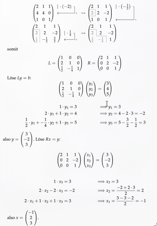
Problem 45: Short tasks
(a) Let \(A \in \mathbb{R}^{N \times N}\) be a regular matrix. If the \(LR\)-decomposition of \(A\) exists, it is unique (\(L\) lower triangular matrix with 1s on the diagonal, \(R\) upper triangular matrix).
(b) Let \(A \in \mathbb{R}^{N \times N}\) be a regular matrix. The \(QR\)-decomposition of \(A\) is unique (\(Q\) orthogonal matrix, \(R\) upper triangular matrix).
(c) The CG method minimizes the residual in the Euclidean norm, while the GMRES method minimizes the energy norm.
(d) The condition of a matrix \(A\) describes the amplification of the relative error of the input data.
Solution
(a) The LR-decomposition yields \(PA=LR\) with a permutation matrix \(P\). This can, for example, be different for \(LR\)-decomposition with and without column pivoting. However, one can also assume that a permutation matrix was excluded in this problem. In that case, the answer is “correct”.
(b) False, you flip the sign of a column in Q and the corresponding row in R, the product QR remains unchanged.
(c) False, its exactly the opposite.
(d) True
Problem 46: Least Square Problem
Given are the 5 pairs of values:
$$ \begin{array}{c|ccccc} i & 0 & 1 & 2 & 3 & 4 \\ \hline t_i & -1 & \tau & 1 & 2 & 4 \\ y_i & 0 & 0 & 4 & 2 & 5 \end{array} $$Let \(g(t) = at + b\) be a polynomial of degree 1 that minimizes the sum of squared errors \(\sum_{i=0}^4 (g(t_i) - y_i)^2\) at the 5 support points.
a) Give the normal equations for this least squares problem, as well as the matrices used explicitly.
b) Now calculate all \(\tau \in (-1,1)\) such that the minimizing line \(g(x)\) has a slope \(a = 1\).
c) For the smallest of these \(\tau\), state the sum of squared errors.
Solution a)
The Normal equation is
$$ A^TAx = A^Tb $$where
$$ A = \begin{pmatrix} -1 & 1 \\ \pi & 1 \\ 1 & 1 \\ 2 & 1 \\ 4 & 1 \end{pmatrix} $$and
$$ A(a \ b)^T = b $$Solution b)
We solve \(A^TAx = A^Tb\), hence
$$ \begin{pmatrix} 22 + \pi & 6 + \pi \\ 6 + \pi & 5 \end{pmatrix} \begin{pmatrix} 1 \\ b \end{pmatrix} =^! \begin{pmatrix} 28 \\ 11 \end{pmatrix} $$which is \(\pi \in \{0, 1/4\}\).
Solution c)
$$ \sum^4 (g(t_i) - y_i)^2 = \sum^4 (t_i + 1 - y_i)^2 = 6 $$Problem 47: Polynomial interpolation
Given the function \(f(t) = t - \cos(\pi t)\) and the support points \(t_0 = -1\), \(t_1 = 0\), \(t_2 = 1\), \(t_3 = 2\). Determine the third-degree interpolation polynomial \(P_3\) for \(f\) with respect to the support points.
a) in Newton form
In particular, specify the corresponding basis.
Solution a)
Given the values:
$$f(t_0) = -1 - \cos(-\pi) = 0$$$$f(t_1) = 0 - \cos(0) = -1$$$$f(t_2) = 1 - \cos(\pi) = 2$$$$f(t_3) = 2 - \cos(2\pi) = 1$$In Newton form, the polynomial is given with respect to the Newton basis
$$\{1, x-t_0, (x-t_0)(x-t_1), (x-t_0)(x-t_1)(x-t_2)\}$$The divided differences are calculated as follows:
$$f[t_0] = 0$$$$f[t_0, t_1] = \frac{f[t_1] - f[t_0]}{t_1 - t_0} = \frac{-1 - 0}{0 - (-1)} = -1$$$$f[t_1, t_2] = \frac{f[t_2] - f[t_1]}{t_2 - t_1} = \frac{2 - (-1)}{1 - 0} = 3$$$$f[t_2, t_3] = \frac{f[t_3] - f[t_2]}{t_3 - t_2} = \frac{1 - 2}{2 - 1} = -1$$$$f[t_0, t_1, t_2] = \frac{f[t_1, t_2] - f[t_0, t_1]}{t_2 - t_0} = \frac{3 - (-1)}{1 - (-1)} = 2$$$$f[t_1, t_2, t_3] = \frac{f[t_2, t_3] - f[t_1, t_2]}{t_3 - t_1} = \frac{-1 - 3}{2 - 0} = -2$$$$f[t_0, t_1, t_2, t_3] = \frac{f[t_1, t_2, t_3] - f[t_0, t_1, t_2]}{t_3 - t_0} = \frac{-2 - 2}{2 - (-1)} = -\frac{4}{3}$$The interpolation polynomial in Newton form is therefore:
$$ - (x+1) + 2(x+1)x - \frac{4}{3}(x+1)x(x-1)$$Problem 48: Splines
Given the function \(f(t) = \sin(\pi t)\) and the support points \(t_0 = -2, t_1 = -1, t_2 = 0, t_3 = 1, t_4 = 2\). Provide a cubic spline that interpolates this function at the support points. Show that your solution also satisfies the properties of an interpolating cubic spline.
Solution
The splines needs to fulfill
$$ p(x_n) = y_n, \quad p_{|x_n; x_{n+1}} $$We first calculate the function values
$$ f(-2) = f(-1) = f(0) = f(1) = f(2) = 0 $$This means the \(f\) is interpolated by \(p(x)=0\), because \(f(x_n)=y_n\) and it can be derived two times.
It fulfills the property of being periodic as \(f'(a) = f'(b) = 0\) and \(f''(a) = f''(b) = 0\).
Problem 49: QR-Decomposition
Calculate the \(QR\)-decomposition of
$$A = \begin{pmatrix} 1 & 2 \\ 1 & 2 \\ \sqrt{2} & \sqrt{2} \end{pmatrix}.$$In doing so, give all used Householder transformations \(Q\).
Solution
We start by defining our initial vector
$$ a^1 = \begin{pmatrix} 1 \\ 1 \\ \sqrt{2} \end{pmatrix} $$Next we calculate \(w\)
$$ w^1 = a^1 + |a^1|_2 e^1 = a^1 + 2 e^1 = \begin{pmatrix} 3 \\ 1 \\ \sqrt{2} \end{pmatrix} $$To get our householder transformation
$$ Q_1 = I - 2\frac{ww^T}{|ww^T|} = I - \frac{1}{6} ww^T = I - \begin{pmatrix} 9 & 3 & 3\sqrt{2} \\ 3 & 1 & \sqrt{2} \\ 3\sqrt{2} & \sqrt{2} & 2 \end{pmatrix} = \begin{pmatrix} -1/2 & -1/2 & -\sqrt{2}/2 \\ -1/2 & 5/6 & -\sqrt{2}/6 \\ -\sqrt{2}/2 & -\sqrt{2}/6 & 2/3 \end{pmatrix} $$We apply the transformation
$$ Q_1 A = \begin{pmatrix} -2 & -3\\ 0 & 1/3\\ 0 & \frac{-2\sqrt{2}}{3} \end{pmatrix} $$We can now calculate the second householder transformation
$$ a^2 = \begin{pmatrix} 1/3 \\ \frac{-2\sqrt{2}}{3} \end{pmatrix} $$Next
$$ w^2 = a^2 + |a^2|_2 e^1 = a^2 + 1 e^1 = \begin{pmatrix} 4/3 \\ \frac{-2\sqrt{2}}{3} \end{pmatrix} $$We continue
$$ Q_1 = I - 2\frac{ww^T}{|ww^T|} = I - \frac{3}{4} ww^T = \begin{pmatrix} -1/3 & 2\sqrt{2}/3 \\ 2\sqrt{2}/3 & 1/3 \end{pmatrix} $$We apply the second transformations
$$ Q_2 \cdot Q_1 \cdot A = \begin{pmatrix} -2 & -3 \\ 0 & -1 \\ 0 & 0 \end{pmatrix} = R $$And
$$ Q = Q_1 \cdot Q_2 $$Problem 50: Short Answers
a) We consider the norm \(\lVert \cdot \rVert_p\) on \(\mathbb{R}^{N \times N}\) for \(p \in [1, \infty]\). Give the definition for the condition number \(\kappa_p(A)\) and show that \(\kappa_p(A) \ge 1\).
b) Given
$$A = \begin{pmatrix} \alpha & \beta \\ \gamma & \delta \end{pmatrix}$$State the conditions for \(\alpha, \beta, \gamma, \delta \in \mathbb{R}\) such that \(A\) possesses an LR-decomposition (without pivoting). Determine the LR-decomposition in the case of its existence.
c) Given a continuously differentiable function \(F: \mathbb{R}^N \to \mathbb{R}^N\). We consider the nonlinear system of equations \(F(x) = 0\) in \(\mathbb{R}^N\). Formulate one step of the Newton iteration and briefly discuss the efficient calculation of the Newton correction.
d) Given the expression:
$$\sqrt{x^2 + 1} - x \quad \text{for } x \gg 1.$$Explain and fix the problem when evaluating the expression.
e) Name one advantage and one disadvantage of the LR-decomposition compared to the Cholesky decomposition.
f) Iterative computation of eigenvalues:
(i) Explain how the output of the inverse iteration (with shift) and the QR-iteration (with shift) differ after successful execution.
(ii) State how in the inverse iteration one obtains the same sequence of shifts \(\mu_k\) as in the QR-iteration.
Solution a)
For regular matrices we have
$$ K_p(A) = ||A||_p ||A^{-1}||_p $$Next we show that \(K_p(A) \geq 1\)
$$ K_p(A) = ||A||_p ||A^{-1}||_p \geq ||AA^{-1}||_p = ||I_n||_p = 1 $$Solution b)
A LR-decomposition has the following structure
$$ L = \begin{pmatrix} 1 & 0 \\ l_{11} & 1 \end{pmatrix}, \quad R = \begin{pmatrix} r_{11} & r_{12} \\ 0 & r_{22} \end{pmatrix} $$In our case \(r_{11} = \alpha, \ r_{12} = \beta, \ r_{22} = \delta - l_{21}\beta\) and from this follows the last element \(l_{21} = \frac{\gamma}{\alpha}\).
Hence
$$ L = \begin{pmatrix} 1 & 0 \\ \frac{\gamma}{\alpha} & 1 \end{pmatrix}, \quad R = \begin{pmatrix} \alpha & \beta \\ 0 & \delta - l_{21}\beta \end{pmatrix} $$And such a LR-decomposition exist if and only if main minors are ivnertible/regular, this is then the case when the determinant is non zero. Hence
$$ det_1(A) = \alpha , \quad det_2(A) = \alpha \delta - \beta \gamma $$needs to be non-zero.
Alternative LR-Decomposition
$$ \text{LU:} \quad \begin{pmatrix} a & b \\ c & d \end{pmatrix} \;\xrightarrow{\;-\frac{c}{a}\;} \; \begin{pmatrix} a & b \\ 0 & d - \frac{bc}{a} \end{pmatrix} $$$$ \Rightarrow L = \begin{pmatrix} 1 & 0 \\ \frac{c}{a} & 1 \end{pmatrix} \quad \checkmark \qquad U = \begin{pmatrix} a & b \\ 0 & d - \frac{bc}{a} \end{pmatrix} \quad \checkmark $$Solution c)
We have
$$ x^{k+1} = x^{k} = d^{k} $$whereby \(d^k\) is the solution of
$$ DF(x^k) d^k = -F(x^k) $$To calculate this efficiently, instead of caculatign the inverse of the matrix we use an LGS.
Solution d)
The Problem: For very big x are the terms nearly identical big, as such it comes to destruction.
To solve this we need to avoid subtracing two nmumbers that are nearly identical big
$$ \sqrt{x^2+1} - x = \left(\sqrt{x^2+1} - x\right) \frac{\sqrt{x^2+1} + x}{\sqrt{x^2+1} + x} = \frac{(x^2+1) - x^2}{\sqrt{x^2+1} + x} = \frac{1}{\sqrt{x^2+1} + x} $$Solution e)
Advantages:
- Less requirement, choelsky needs spd.
Disadvantages:
- LR Decomposition takes more operation i.e. more expensiver.
Solution f)
(i) in the inverse iteration we get one eigenvalue and its eigenvector. In QR-iteration we get the entire spectrum i.e. all eigenvalues in from of a matrix.
(ii) We start with \(e^N\), that is the N-th unit vector.
Problem 51: Linear Curve fitting
Given the Matrix
$$ A = \begin{pmatrix} 1 & -5 \\ 2 & 0 \\ 2 & 1 \end{pmatrix} $$and a vector \(\mathbf{b} \in \mathbb{R}^3\).
a) Calculate the QR-decomposition of \(A\). Hint: For \(Q\), it is sufficient to provide a formula.
b) Define the linear least squares problem for \(A\mathbf{x} = \mathbf{b}\) and check whether it has a unique solution.
c) Explain how you could solve the least squares problem from part b) using the result from part a).
Solution a)
Step 1:
$$ a^1 = \begin{pmatrix} 1 \\ 2 \\ 2 \end{pmatrix}, \quad w^1 = \begin{pmatrix} 1 \\ 2 \\ 2 \end{pmatrix} + |a^1|_2 \cdot e^1 = \begin{pmatrix} 4 \\ 2 \\ 2 \end{pmatrix} $$Further \(|w_1|^2_2 = 24\), hence we become the householder matrix
$$ Q = I - 2 \frac{ww^T}{w^Tw} = I- \frac{1}{12} \begin{pmatrix} 16 & 8 & 8 \\ 8 & 4 & 4 \\ 8 & 4 & 4 \end{pmatrix} = \frac{1}{3} \begin{pmatrix} -1 & -2 & -2 \\ -2 & 2 & -1 \\ -2 & -1 & 2 \end{pmatrix} $$We apply the householder matrix
$$ Q_1 \cdot A = \begin{pmatrix} -3 & 1 \\ 0 & 3 \\ 0 & 4 \end{pmatrix} $$Step 2:
$$ a^2 = \begin{pmatrix} 3 \\ 4 \\ \end{pmatrix}, \quad w^2 = \begin{pmatrix} 3 \\ 4 \\ \end{pmatrix} + |a^2|_2 \cdot e^1 = \begin{pmatrix} 9 4 \end{pmatrix} $$Further \(|w^2|^2_2 = 80\). We get the second housholder matrix
$$ \hat{Q}_2 = I - 2 \frac{ww^T}{w^Tw} = I- \frac{1}{40} \begin{pmatrix} 64 & 32 \\ 32 & 16 \\ \end{pmatrix} = \frac{1}{5} \begin{pmatrix} -3 & -4 & \\ -4 & 3 & \\ \end{pmatrix} $$And with
$$ Q_2 = \begin{pmatrix} 1 & \\ & \hat{Q}_2 \end{pmatrix} $$We get
$$ R = Q_2 \cdot Q_1 \cdot A = \begin{pmatrix} -3 & 1 \\ 0 & - 5 \\ 0 & 0 \end{pmatrix} $$And
$$ Q = Q_1 \cdot Q_2 $$Solution b)
The linear least square/curve fitting problem is defined as
$$ \min_x \ |Ax - b|_2 $$This problem is then exact solvable when A has full rank. In our case, since the columns are linear independent this is the case and the problem has one unique solution.
Solution c)
From the lecture we know that the normal equation solves a linear least square problem
$$ A^TAb = A^Tb $$We can now use the QR-decomposition, by inserting them in our equation
$$ (QR)^T(QR)b = R^TQ^TQRb = R^TRb = A^Tb $$which can be solved using forward and backward substitution.
Problem 52: Polynomial Interpolation
Given the table of values:
$$ \begin{array}{|c|c|c|c|c|} \hline n & 0 & 1 & 2 & 3 \\ \hline \xi_n & -3 & -1 & 1 & 2 \\ \hline f_n & 3 & -1 & -5 & 12 \\ \hline \end{array} $$a) Determine the interpolation polynomial \(P \in \mathbb{P}_3\) such that \(P(\xi_n) = f_n\) for \(n=0, 1, 2, 3\) in the Newton form (or Newton basis).
b) Extend the interpolation polynomial by including the point \((\xi_4, f_4) = (0, 0)\).
c) Briefly justify whether the calculated interpolation polynomials in parts a) and b) are unique.
Solution a)
The Neville Scheme is:
$$ \begin{array}{c|c|ccc} \xi_n & f_n & P_{0,1} & P_{0,1,2} & P_{0,1,2,3} \\ \hline -3 & 3 & & & \\ -1 & -1 & \frac{-1 - 3}{-1 - (-3)} = -2 & & \\ 1 & -5 & \frac{-5 - (-1)}{1 - (-1)} = -2 & \frac{-2 - (-2)}{1 - (-3)} = 0 & \\ 2 & 12 & \frac{12 - (-5)}{2 - (1)} = 17 & \frac{17 - (-2)}{2 - (-1)} = \frac{19}{3} & \frac{\frac{19}{3} - 0}{2 - (-3)} = \frac{19}{15} \\ \end{array} $$Thus, the interpolation polynomial in Newton form is:
$$P_1(t) = 3 - 2(t+3) + 0(t+3)(t+1) + \frac{19}{15}(t+3)(t+1)(t-1)$$Solution b)
$$ \begin{array}{c|c|cccc} \xi_n & f_n & \text{1st Diff.} & \text{2nd Diff.} & \text{3rd Diff.} & \text{4th Diff.} \\ \hline -3 & 3 & & & & \\ -1 & -1 & \frac{-1 - 3}{-1 - (-3)} = -2 & & & \\ 1 & -5 & \frac{-5 - (-1)}{1 - (-1)} = -2 & \frac{-2 - (-2)}{1 - (-3)} = 0 & & \\ 2 & 12 & \frac{12 - (-5)}{2 - (1)} = 17 & \frac{17 - (-2)}{2 - (-1)} = \frac{19}{3} & \frac{\frac{19}{3} - 0}{2 - (-3)} = \frac{19}{15} & \\ \hline \mathbf{0} & \mathbf{0} & \mathbf{\frac{0 - 12}{0 - 2} = 6} & \mathbf{\frac{6 - 17}{0 - 1} = 11} & \mathbf{\frac{11 - \frac{19}{3}}{0 - (-1)} = \frac{14}{3}} & \mathbf{\frac{\frac{14}{3} - \frac{19}{15}}{0 - (-3)} = \frac{51}{45} \left(= \frac{17}{15}\right)} \\ \end{array} $$Hence
$$ P_2(t) = P_1(t) + \frac{17}{15} (t + 3)(t + 1)(t -1)(t - 2) $$Solution c)
Because the polynomial has n-th degree, it is uniquely determined by n-points, hence the solution is unique.Problem 53: Quadratur
We consider the interval \(I = [a, b]\) for \(a, b \in \mathbb{R}\) and \(a < b\).
a) Given are the nodes \(\xi_0 = a, \xi_1 = b\) and the weights \(\omega_0 = \omega_1 = \frac{b-a}{2}\).
(i) Show that the given quadrature formula is exact for all polynomials \(P \in \mathbb{P}_1\).
(ii) Show that the given quadrature formula is no longer exact for polynomials \(P \in \mathbb{P}_2\). Hint: A counterexample is sufficient.
b) Given are \(f \in C^2[a, b]\) as well as the equidistant nodes
$$\xi_n = a + n h \quad \text{for } n = 0, \ldots, N, \quad h = \frac{b-a}{N}.$$The composite (right-sided) rectangle rule is defined by
$$Q(f) = \sum_{n=1}^{N} h f(\xi_n).$$(i) Show the error estimate
$$\left| \int_a^b f(t) \, dt - Q(f) \right| \leq \frac{b-a}{2} h \sup_{t \in [a, b]} |f'(t)|.$$(ii) Briefly explain how you can improve the order of the error of \(Q(\cdot)\) with the help of an additional function evaluation. Give the improved, composite quadrature formula explicitly and name it.
Solution a)
(i) Recall:
$$ Q_T(f) \sum_\xi w_\xi f(\xi) $$For the quadrature to be exact, the following needs to be true
$$ \forall P \in \mathbb{P}_1 : \int_a^b P(x) dx = Q_T(P) $$We can show that, by showing it for the monom base \(1, x \in \mathbb{P}_1\)
$$ \int^b_a 1 dx = [x]^b_a = b - a = \frac{b - a}{2} (1 + 1) = Q_T(1) $$$$ \int^b_a x dx = [\frac{1}{2}x^2]^b_a = \frac{b^2 - a^2}{2} = \frac{b - a}{2}(b - a) $$As such is \(Q_T\) exact for \(\mathbb{P}_1\).
(ii)
We choose \(a=0, b=1\) then
$$ \int^1_0 x^2 dx = [\frac{1}{3}x^3]^1_0 = \frac{1}{3} \neq \frac{1}{2} = \frac{1- 0}{2}(1^2 - 0^2) = Q_T(x^2) $$Solution b)
(i) We do a taylor development for \(f\) with \(t_n \in [\xi_{n-1}, \xi_n]\)
$$ f(t) = f(\xi_n) + f'(t_n)(t - \xi_n) $$With that we can begin
$$ \begin{align} \int^b_a f(t) dt - Q(f) &= \int^b_a f(t) dt - \sum_{n = 1}^{N} h f(\xi_n) \\ &= \sum_{n = 1}^{N}(\int_{\xi_{n-1}}^{\xi_n} f(t) dt) - \sum_{n = 1}^{N} h f(\xi_n) \\ &= \sum_{n = 1}^{N} (\int_{\xi_{n-1}}^{\xi_n} f(t)dt - hf(\xi_n)) \\ &= \sum_{n = 1}^{N} (\int_{\xi_{n-1}}^{\xi_n} f(\xi_n) + f'(t_n)(t - \xi_n)dt - hf(\xi_n)) \\ &= \sum_{n = 1}^{N} (\int_{\xi_{n-1}}^{\xi_n} f(\xi_n) + \int_{\xi_{n-1}}^{\xi_n} f'(t_n)(t - \xi_n)dt - hf(\xi_n)) \\ &= \sum_{n = 1}^{N} ( f(t)[C]^{\xi_{n-1}}_{\xi_n} + f'(t_n) [t - \xi_n]^{\xi_{n-1}}_{\xi_n} - hf(\xi_n)) \\ &= \sum_{n = 1}^{N} ( hf(t) - f'(t_n) \frac{1}{2}h^2 - hf(\xi_n)) \\ &= \sum_{n = 1}^{N} - f'(t_n) \frac{1}{2}h^2 \\ &= -\frac{h}{2} \sum_{n = 1}^{N} \frac{b - a}{N}f'(t_n) \\ &\leq -\frac{h}{2} \sum_{n = 1}^{N} \frac{b - a}{N} \sup_{t \in [a, b]}f'(t) \\ &= \frac{h}{2} \sup_{t \in [a, b]}f'(t) \sum_{n = 1}^{N} \frac{b - a}{N} \\ &= \frac{b-a}{2}h \sup_{t \in [a, b]}f'(t) \end{align} $$Explanations:
- From Line 1 to 2: Split the integral over \([a,b]\) into the sum of the integrals on the subintervals \([\xi_{n−1}, \xi_n]\).
- From Line 2 to 3: Then group each subinterval’s integral with the corresponding right-endpoint rectangle \(hf(\xi_n))\).
- From Line 3 to 4: Insert the taylor development
- From Line 4 to 7: Integrate the summands independent
- From Line 7 to 8: \(hf(\xi)\) cancels each other out.
- From Line 8 to 9: Replace one \(h\) by its definition, pull the other before the sum.
(ii) We can do an additional evaluation, and get the summed trapezoid rule. From the lecture we know that its error order is 2.
$$ Q(f) = \frac{f(a) + f(b)}{2} + \sum_{n=1}^{N-1} h f(\xi_n) $$Problem 54: Linear Iteration Method
We consider the linear system of equations \(A\mathbf{x} = \mathbf{b}\) for \(A \in \mathbb{R}^{N \times N}\) and \(\mathbf{b} \in \mathbb{R}^N\).
a) State the formula (or prescription) for a general linear iterative method and name the quantities involved.
Let’s now specifically consider
$$ A = \begin{pmatrix} \alpha & \beta \\ \gamma & \delta \end{pmatrix} $$for \(\alpha, \beta, \gamma, \delta \in \mathbb{R}_{>0}\) (i.e., all entries are strictly positive).
b) Determine the conditions on \(\alpha, \beta, \gamma, \delta\) such that, for arbitrary starting vectors \(\mathbf{x}^{(0)} \in \mathbb{R}^2\) and right-hand sides \(\mathbf{b} \in \mathbb{R}^2\):
(i) the Jacobi method converges for \(A\).
(ii) the Gauss-Seidel method converges for \(A\).
Solution a)
Let \(B\) be a pre-conditioning matrix, then the iteration method is given by
$$ x^{k+1} = x^k + B(b-Ax^k) $$where \(x^k\) the iterative is of the method.
Alternative:
- Choose \(\mathbf{x}^{(0)}\) and \(\varepsilon\).
- While \(\Vert \mathbf{r}^{(k)} \Vert < \varepsilon \Vert \mathbf{b} \Vert\)
- Calculate $$ \begin{aligned} \mathbf{c}^{(k)} &= B \mathbf{r}^{(k)} \\ \mathbf{x}^{(k+1)} &= \mathbf{x}^{(k)} + \mathbf{c}^{(k)} \\ \mathbf{r}^{(k+1)} &= \mathbf{r}^{(k)} - A \mathbf{c}^{(k)} \end{aligned} $$ where \(A = L + D + R\). E.g., in Jacobi: \(\mathbf{B} = \mathbf{D}^{-1}\). \(\mathbf{r}^{(k)}\) is the residual, \(\mathbf{x}^{(0)}\) is the starting vector, \(\varepsilon\) determines how large the error of our final result is.
Solution b)
From the Lecture we know a generel linear iteration method converges with start vector \(x^0\) when \(p(I - BA) \le 1\).
(i) For Jacobi-Method we have \(B = D^{-1}\) and hence
$$ C_1 = I - BA = I - \begin{pmatrix} \alpha^{-1} & 0 \\ 0 & \delta^{-1} \end{pmatrix} A = \begin{pmatrix} 0 & -\frac{\beta}{\alpha} \\ -\frac{\gamma}{\delta} & 0 \end{pmatrix} $$We calculate the characteristic polynomial
$$ det(\lambda I_N - C_1) = det( \begin{pmatrix} \lambda & \frac{\beta}{\alpha} \\ \frac{\gamma}{\delta} & \lambda \end{pmatrix} ) = \lambda^2 - \frac{\beta\gamma}{\alpha \delta} $$The roots of this are \(\lambda_{1,2} \pm \sqrt{\frac{\beta\gamma}{\alpha \delta}}\).
This means for the method to converge \(|\lambda_{1,2}| < 1\) needs to be true, this is the case when \(\beta \gamma < \alpha \delta\).
(ii) For Gauß-Seidel-Method we have \(B = (L + D)^{-1}\) and hence
$$ B = \begin{pmatrix} \alpha^{-1} & 0 \\ -\frac{\gamma}{\delta} & \delta^{-1} \end{pmatrix} $$With this we have
$$ C_2 = I - BA = \begin{pmatrix} 0 & -\frac{\beta}{\alpha}\\ 0 & \frac{\beta\gamma}{\alpha\delta} \end{pmatrix} $$We calculate the characteristic polynomial
$$ det(\lambda I_N - C_2) = det( \begin{pmatrix} \lambda & -\frac{\beta}{\alpha}\\ 0 & \lambda - \frac{\beta\gamma}{\alpha\delta} \end{pmatrix} ) = \lambda(\lambda - \frac{\beta\gamma}{\alpha\delta}) $$The roots of this are \(\lambda_{1} = 0 \) and \(\lambda_{2} = \frac{\beta\gamma}{\alpha\delta}\).
This means for the method to converge \(|\lambda_{1,2}| < 1\) needs to be true, this is the case when \(\beta \gamma < \alpha \delta\).
Problems with Non-Confirmed Solution
Problem 55: Iterations method
Given
$$ A = \begin{pmatrix} 2 & 1 & 1 \\ 4 & 4 & 0 \\ 1 & 0 & 2 \end{pmatrix}, \quad b = \begin{pmatrix} 3 \\ 4 \\ 5 \end{pmatrix} $$a) Give step for step the algorithm for the Geis-Seidel iteration algorithm.
Solution a)
- \(A = L + D + R\) with \(B = L + D\)
- Choose \(\epsilon, x_0\)
- For as long \(||r^k|| < \epsilon ||b||\)
- Calculate $$ Bc^k = r^k x^{k+1} = x^k + c^k r^{k+1} = r^k - Ac^k $$
Problem 56: Short tasks
(a) Explain briefly why the evaluation of the term \(\sqrt{x + \frac{1}{x}} - \sqrt{x - \frac{1}{x}}\) on a computer with floating-point arithmetic is problematic for \(x \gg 1\). Transform the term so that this problem no longer occurs.
(b) We consider the set of normalized floating-point numbers FL with base \(B\) and mantissa length \(M\). Give the floating-point representation of the number 1 in FL and the smallest number \(x \in \text{FL}\) with \(x > 1\). Hint: Give the mantissa and the exponent explicitly in each case.
(c) Justify why the two given matrices \(A\) and \(B\) cannot be Givens rotations.
$$A = \begin{pmatrix} 1/2 & \sqrt{3}/2 & 0 \\ -\sqrt{3}/2 & 1/2 & 0 \\ 0 & 0 & -1 \end{pmatrix}, \quad B = \begin{pmatrix} 1/2 & -\sqrt{3}/2 & 1/4 \\ -\sqrt{3}/2 & 1/2 & 1/4 \\ 1/2 & 1/2 & 1/2 \end{pmatrix}$$(d) Calculate \(\|A\|_{\infty}\) and \(\|A\|_1\) for \(A = \begin{pmatrix} 4 & -3 & -2 \\ -1 & 0 & 1 \\ -2 & 3 & 5 \end{pmatrix}\).
(e) Let \(A \in \mathbb{R}^{N \times N}\) be regular and \(\alpha \in \mathbb{R} \setminus \{0\}\). Determine the condition \(\kappa(\alpha A)\) in dependence on \(\kappa(A)\).
(f) Let \(A, B \in \mathbb{R}^{N \times N}\) be regular and let \(\mathbf{b} \in \mathbb{R}^N\). Show: If the iteration method \(\mathbf{x}^{k+1} = \mathbf{x}^k + B( \mathbf{b} - A\mathbf{x}^k)\) converges, then it converges against \(A^{-1}\mathbf{b}\). Additionally, state a sufficient condition for the linear convergence of the method.
(g) Let \(f: \mathbb{R}^N \to \mathbb{R}\) be a twice continuously differentiable function. Formulate Newton’s method for solving the minimization problem \(\min_{\mathbf{x} \in \mathbb{R}^N} f(\mathbf{x})\).
Solution a)
Because if \(x >> 1\), then the terms we subtract are nearly identical and it thus comes to extinction.
$$ \sqrt{x + \frac{1}{x}} - \sqrt{x - \frac{1}{x}} = \frac{(\sqrt{x + \frac{1}{x}} - \sqrt{x - \frac{1}{x}})(\sqrt{x + \frac{1}{x}} - \sqrt{x - \frac{1}{x}})}{(\sqrt{x + \frac{1}{x}} - \sqrt{x - \frac{1}{x}})} = \frac{2}{x(\sqrt{x + \frac{1}{x}} + \sqrt{x - \frac{1}{x}})} $$Solution b)
Floating point number
$$ m \cdot B^e : m = \sum^{L_m} c_i B^{-l}, \ e = e_{min} + \sum^{L_e} a_l B^{l} $$1-Number : \((1 B^{-0})B^1\)
Addition: Smallest positive number in general \(B^{e_{min} - 1}\)
Solution c)
A givens rotations looks like this
$$ \begin{pmatrix} c & c \\ -s & c \end{pmatrix} $$and \(c^2 + s^2 = 1\) which is also fulfilled.
But the matrices are not orthogonal \(E = Q^TQ\).
Solution d)
The sum of the first column is 7. The sum of the second column is 6. The sum of the third column is 8.
Hence the result is 8.
Solution e)
$$ K(\alpha A) = ||\alpha A|| ||\alpha^{-1} A^{-1} || = ||A|| ||A^{-1} || +K(A) $$Solution f)
$$ (b - Ax^k) = 0 \iff Ax^k = b \iff x^k A^{-1}b $$Solution g)
$$ x^{k+1} = x^k + d^k $$with
$$ f''(x)d^k = -f'(x) $$Problem 57: Decompositions
Given:
$$A_{\alpha,\beta} = \begin{pmatrix} 4 & \beta & 1 \\ \alpha & 2 & 0 \\ 1 & 0 & 1 \end{pmatrix}, \quad \alpha, \beta \in \mathbb{R}, \quad \mathbf{b} = \begin{pmatrix} -4 \\ -6 \\ 2 \end{pmatrix}$$(a) Determine all \(\alpha, \beta \in \mathbb{R}\) for which a Cholesky decomposition of \(A_{\alpha,\beta}\) exists, using the principal minors criterion.
(b) Calculate the \(LR\)-decomposition of \(A_{2,6}\). Give the matrices \(L\) and \(R\) explicitly with \(A_{2,6} = LR\).
(c) Determine the solution of the linear system \(A_{4,0}\mathbf{x} = \mathbf{b}\) using \(A_{4,0} = LR\) with
$$L = \begin{pmatrix} 1 & 0 & 0 \\ 1 & 1 & 0 \\ \frac{1}{4} & 0 & 1 \end{pmatrix}, \quad R = \begin{pmatrix} 4 & 0 & 1 \\ 0 & 2 & -1 \\ 0 & 0 & \frac{3}{4} \end{pmatrix}.$$(d) Give the general iteration formula for the single-step method (Gauss-Seidel method) in matrix notation.
Solution a)
Choleksy exist if spd, it is symmetrical when \(\alpha = \beta\).
And positive definite if \(\alpha < \sqrt{6}\)
Solution b)
$$ A = LR \iff \begin{pmatrix} 4 & 6 & 1 \\ 2 & 2 & 0 \\ 1 & 0 & 1 \end{pmatrix} = \begin{pmatrix} 1 & 0 & 0 \\ \frac{1}{2} & 1 & 0 \\ \frac{1}{4} & \frac{3}{2} & 1 \end{pmatrix} \cdot \begin{pmatrix} 4 & 6 & 1 \\ 0 & -1 & -\frac{1}{2} \\ 0 & 0 & \frac{3}{2} \end{pmatrix} $$Solution c)
- From the first row: \(1 \cdot y_1 = -4 \implies y_1 = -4\).
- From the second row: \(1 \cdot y_1 + 1 \cdot y_2 = -6\). Substituting \(y_1 = -4\), we get \((-4) + y_2 = -6 \implies y_2 = -2\).
- From the third row: \(\frac{1}{4} \cdot y_1 + 0 \cdot y_2 + 1 \cdot y_3 = 2\). Substituting \(y_1 = -4\), we get \(\frac{1}{4}(-4) + y_3 = 2 \implies -1 + y_3 = 2 \implies y_3 = 3\).
So, the intermediate vector is \(\mathbf{y} = \begin{pmatrix} -4 \\ -2 \\ 3 \end{pmatrix}\).
- From the third row: \(\frac{3}{4} \cdot x_3 = 3 \implies x_3 = 3 \cdot \frac{4}{3} = 4\).
- From the second row: \(2 \cdot x_2 - 1 \cdot x_3 = -2\). Substituting \(x_3 = 4\), we get \(2x_2 - 4 = -2 \implies 2x_2 = 2 \implies x_2 = 1\).
- From the first row: \(4 \cdot x_1 + 0 \cdot x_2 + 1 \cdot x_3 = -4\). Substituting \(x_3 = 4\), we get \(4x_1 + 4 = -4 \implies 4x_1 = -8 \implies x_1 = -2\).
Therefore, the solution to the linear system \(A_{4,0}\mathbf{x} = \mathbf{b}\) is \(\mathbf{x} = \begin{pmatrix} -2 \\ 1 \\ 4 \end{pmatrix}\).
Solution d)
Do until \(||r^k|| < \epsilon ||b||\)
$$ Bc^k = r^k, \quad x^{k+1} = x^k + c^k, \quad r^{k+1} = r^k - Ac^k $$with \(A = L + D + R\) and \(B = L + D\)
Problem 58: QR-Algorithm
We consider the \(QR\)-algorithm with variable shift for the simultaneous computation of all eigenvalues of a symmetric matrix \(A \in \mathbb{R}^{N \times N}\).
(a) Explain how the starting matrix \(A_0\) is calculated and state the asymptotic computational cost (\(O(\cdot)\)) for this calculation.
(b) State how, in one iteration, the matrix \(A_{k+1}\) is calculated from the matrix \(A_k\) and the shift \(\mu_k\).
(c) Show that all iterates \(A_k\) in the \(QR\)-algorithm have the same eigenvalues.
(d) Briefly explain why the starting matrix \(A_0\) used in the algorithm is advantageous compared to \(A\) for an efficient execution of the algorithm.
(e) State the asymptotic computational cost of one step of the algorithm.
Solution a)
We transform \(A\) first into its Hessenbergform. The algorithm then takes \(O(N^3)\).Solution b)
$$ QR = A_k - \mu I $$and
$$ A_{k+1} = RQ + \mu I $$Solution c)
$$ A_{k+1} = RQ + \mu I = Q^T(R + \mu)Q_k + \mu I = Q^TAQ $$Thus we do in every step a orthogonal transformation, which leave eigenvalues intact.
Solution d)
Its faster.Solution e)
$$ O(N) $$Problem 59: Interpolation polynomial
Let \(\xi_0 < \xi_1 < \dots < \xi_N\) and \(f_0, f_1, \dots, f_N \in \mathbb{R}\) be given.
(a) Formulate the interpolation problem for the data \((\xi_n, f_n), n=0, \dots, N\).
(b) Give the Newton basis of \(\mathbb{P}_N\) for the nodes \(\xi_0, \dots, \xi_N\).
(c) Use divided differences to compute the interpolation polynomial \(P_2(t)\) for the following data:
$$ \begin{array}{c|ccc} n & 0 & 1 & 2 \\ \hline \xi_n & \frac{1}{2} & 1 & 2 \\ f_n & -1 & 0 & \frac{1}{2} \end{array} $$Hint: The monomial form of \(P_2(t)\) is not required.
(d) Instead of \(\xi_3 = 3\), an additional value \(f_3 = -1\) is given. Compute the new interpolation polynomial \(P_3(t)\).
(e) Name two disadvantages of the Lagrange form of the solution to the interpolation problem.
Solution a)
We want to find a polynomial for that is
$$ p(x_n) = f_n $$Solution b)
$$ p(x) = \prod (x - x_i) $$Solution c)
$$ \begin{array}{c|c|c|cc} n & \xi_n & f_n \\ \hline 0 & 1 & -1 \\ 1 & 3/2 & 0 & f[\xi_0, \xi_1] = \frac{-1-0}{1-3/2} = 2 \\ 2 & 2 & 1/2 & f[\xi_1, \xi_2] = \frac{0-1/2}{3/2-2} = 1 & f[\xi_0, \xi_1, \xi_2] = \frac{2-1}{1-2} = -1 \end{array} $$$$ P_2(t) = -1 + 2(\xi-1) - 1(\xi-1)(\xi-3/2) $$Solution d)
$$ \begin{array}{c|c|c|ccc} n & \xi_n & f_n \\ \hline 0 & 1 & -1 \\ 1 & 3/2 & 0 & f[\xi_0, \xi_1] = \frac{-1-0}{1-3/2} = 2 \\ 2 & 2 & 1/2 & f[\xi_1, \xi_2] = \frac{0-1/2}{3/2-2} = 1 & f[\xi_0, \xi_1, \xi_2] = \frac{2-1}{1-2} = -1 \\ 3 & 3 & -1 & f[\xi_2, \xi_3] = \frac{1/2-(-1)}{2-3} = -\frac{3}{2} & f[\xi_1, \xi_2, \xi_3] = \frac{1-(-3/2)}{3/2-3} = -\frac{5}{3} & f[\xi_0, \xi_1, \xi_2, \xi_3] = \frac{-1-(-5/3)}{1-3} = -\frac{1}{3} \end{array} $$$$P_3(t) = -1 + 2(\xi-1) - 1(\xi-1)(\xi-3/2) - \frac{1}{3}(\xi-1)(\xi-3/2)(\xi-2)$$Solution e)
- The evaluation is harder
- if we get a new root point, we need to recalculate everything
Problem 60: Integrating
We consider an interval \([a, b] \subset \mathbb{R}\) and the integral \(\int_a^b f(t)dt\) for \(f: [a, b] \to \mathbb{R}\).
(a) Give the general form of a quadrature formula for the approximation of the integral.
(b) State the formula from the lecture for calculating the weights and briefly explain the quantities that appear.
(c) Explain why composite quadrature formulas, such as the composite trapezoidal rule, are used by referring to the error bound of the composite trapezoidal rule and the error bound from (c).
Solution a)
$$ Q_n = (a-b) \sum b_k f(a + c_k(b-a)) $$Solution b)
$$ \frac{1}{q} = \sum c^{q-1}b_k $$where \(q = p + 1\) with \(p\) the maixmal order.
Solution c)
Has a better error.Oral Problems
Problem 61
Let \(Ax = b\) a LGS with \(A \in \mathbb{R}^{n \times n}\) regular and \(b \in \mathbb{R}^{n}\).
Let \(B \sim A^{-1}\) a pre-condition to \(A\). What is the iterations method of a LGS with pre condiiton.
Solution
Our LGS with pre condition is \(BA = Bb\) adn the iteration method
$$ x^{k+1} = x^k + B(b - Ax^k) $$Let \(Ax = b\) a LGS with \(A \in \mathbb{R}^{n \times n}\) regular and \(b \in \mathbb{R}^{n}\).
Let concretely
$$A = \begin{pmatrix} 3 & 1 & 0 \\ 1 & 2 & 0 \\ 0 & 0 & 1 \end{pmatrix}$$Investigate the Jacobi method applied to \(Ax=b\) with the given \(A\), arbitrary right-hand side \(b \in \mathbb{R}^N\) and arbitrary starting vector \(x^0 \in \mathbb{R}^N\) for convergence in the Euclidean norm \(|| \cdot ||_2\).
Solution
We have then linear convergence if
$$ p(I_N -BA) < 1 $$Because we use Jacobi method \(A = L + D + R\) where \(B = D^{-1}\) with
$$ B = \begin{pmatrix} \frac{1}{3} & 0 & 0 \\ 0 & \frac{1}{2} & 0 \\ 0 & 0 & 1 \end{pmatrix} $$And
$$ C = I - BA = \begin{pmatrix} 0 & -1/3 & 0 \\ -1/2 & 0 & 0 \\ 0 & 0 & 0 \end{pmatrix} $$Further
$$ det(\lambda I_n - C) = det( \begin{pmatrix} \lambda & -1/3 & 0 \\ -1/2 & \lambda & 0 \\ 0 & 0 & \lambda \end{pmatrix} ) = \lambda \begin{pmatrix} \lambda & -1/3 \\ -1/2 & \lambda \\ \end{pmatrix} = \lambda (\lambda^2 - 1/6) ) $$We have \(\lambda_1 = 0, \lambda_{2,3} \pm \frac{1}{\sqrt{6}}\), which are all smaller as \(1\), thus it converges.
Rewrite
$$\frac{1}{1+2x} - \frac{1-x}{1+x} \quad \text{for } |x| \ll 1$$so that the expression is well-conditioned in floating-point arithmetic. Briefly justify why the new term is well-conditioned.
Solution
$$ \frac{1}{1 + 2x} - \frac{1-x}{1 + x} = \frac{1+ x - (1-x)(1+ 2x)}{(1 + x)(1+2x)} = \frac{2x^2}{(1+x)(1+2x)} $$What is least quare problem?
Solution
It is defined as
$$ Search \ x \in \mathbb{R}^n \ with \ |Ax - b|_2 = min! $$We do this when we cant solve \(Ax = b\) directly and thus instead solve it approximately.
How can we solve this?
Solution
Using the normal equation
$$ A^TAx = A^Tb $$we get this by taking our least square problem to the power of two.
How can we solve the normal equation?
Solution
We can use the singular decomposition.
$$ A^TA = V \Sigma U^T $$Problem 62
- What is the Raleigh-Constant ?
Solution
Is defined as
$$ r(A, x) = \frac{x^TAx}{x^Tx} $$it approximates eigenvalues.
We can use it as startvalue in inverse iteration with shift.
- What is the Kylov method?
Solution
Also known as cg method. It is an iterative method to solve sparse LGS.- What is a matrixnorm?
Solution
We have defined the associated matrixnorm as
$$ ||X||_A = \sup{x \neq 0} \frac{ ||xX||_A}{||x||} $$A norm is general has three attributes
- Positive definite $$||A|| > 0$$
- Triangle inequality $$||AB|| > ||A||||B||$$
- Homogeneous $$||\lambda A|| = |\lambda|||A||$$
- Calculate for \(z = (1 \ -1 \ 1)^T\) the value of norm \(A\) with $$ A LL^T, \quad L = \begin{pmatrix} 1 & 0 & 0 \\ -2 & 1 & 0 \\ 1 & 0 & 1 \end{pmatrix} $$
Solution
It can be calculated with
$$ z^T LL^T z $$- What is Destruction?
Solution
If we subtract two numbers from wach other which are nearly identical the most significant digits will become 0, while the least significant digits will counts, this leads to a result that is very inaccurate, the number explodes in size.- What is Singular Value Decomposition?
Solution
If we have a matrix A then the singular value decomposition is
$$ A = V \sigma U^T, \quad \sigma = diag(\sigma_1, ..., \sigma_n), \quad \sigma_1 = \sqrt{\lambda_i} $$- Determine the solution of the problem $$|Ax^* -b| = \min |Ax-b|$$ with the help of singular value decomposition
Solution
This can be solved using the normal equation
$$ A^TAx = A^Tb $$which we can express using the singular value decomposition
$$ (V \sigma U^T)^T (V \sigma U^T)x = (V \sigma U^T)^Tb \iff U \sigma V V \sigma Ux = U \sigma V b \iff x^* = U \sigma^{-1} $$- What is the lagrange basis? And why are the solution always unique?
Solution
$$ P(x) = \sum f_n L_n (x), \quad L_n = \prod_{n \neq m} \frac{x - x_n}{x_n - x_m} $$They are always 0, except where the roots are, there they are 1, we multiply that than with the function value at that place.
Suppose there are two polynomials ( p(x) ) and ( q(x) ) of degree ≤ n that both satisfy
$$ p(x_i) = q(x_i) = y_i \quad \forall i. $$Consider their difference:
$$ r(x) = p(x) - q(x). $$Then:
- ( r(x) ) is also a polynomial of degree ≤ n,
- and ( r(x_i) = 0 ) for all ( i = 0, \ldots, n. )
So ( r(x) ) has ( n+1 ) distinct roots (since all ( x_i ) are distinct). But a nonzero polynomial of degree ≤ n can have at most ( n ) roots.
Therefore, ( r(x) ) must be the zero polynomial, i.e. ( p(x) = q(x) ).
- What solve methods did we learn in the lecture?
Solution
- Newton-method: to solve non linear problems.
- Jacobi, Gauß-Seidel method: To solve linear problems.
- What is the QR Algorithm? Why do we do it? Can we speed it up?
Solution
We do it, because the convergence speed it bettert han cholesky but it has more requriemenst. Can be used to solve LGS or to determine eigenvalues like this
$$ A_k = QR A_{k+1} RQ $$We can speed up convergence speed, by starting with an hessian matrix and a shift. To get the hessenbergform we do
$$ H = Q^TAQ $$Problem 63
What is the Tikhonov Regularization? How can it be solved?
Solution
When we have a least square problem \(|Ax - b| = min!\), we cab have the problem that \(A\) has bad condition, which leads to an increase of errors in the solution. To solve this we can use the Tikhonov Regularization, the problem is then formulated as
$$ \frac{1}{2}|Ax - b|^2_2 + \frac{1}{2}\alpha |x|^2_2, \quad \alpha > 0 $$and the solution is
$$ x = (A^TA + \alpha I_n)^{-1}A^Tb $$When choosing \(\alpha\) keep in mind:
- The bigger \(\alpha\), the bigger the approximations error.
- The smaller \(\alpha\), the bigger the conditioning error.
What is the trapezoid rule? What is the summed trapezoid rule? What is the general formula for the quadrature formula? For what are they used?
Solution
Trapezoid rule
$$ \frac{b-a}{2}(f(a) + f(b)) $$Summed Trapezoid rule
$$ T_n(f) = \sum_{n=1}^{N} \frac{b-a}{2}(f(a) + f(b)) $$General formula
$$ Q(f) = \sum w_x f(x) $$They ared use to numericaly solve integrals.
What is the QR-Iteration? How does it work? What do we need to do that QR_iteration gives the same result as the ivnerse iteraiton with shift? What can we do to increase the speed of QR-iteration?
Solution
QR-Iteration is used to find out the eigenvalues.
- Choose \(\mu = A[n,n]\)
- $$ A_k -\mu = Q_kR_k $$
- $$ A_{k+1} = R_kQ_k $$
In inverse shift choose \(v = e^N\).
To increase the speed we transform our matrix \(A\) into hessenbergfrom using \(H = Q^TAQ\).
Problem 64
What is a preconditioning matrix? What is the Jacobi preconditioning matrix? What is an example of a preconditioning matrix?
Solution
A preconditioning matrix \(B\), gets multiplied to our LGS in order to have better conditioning
$$ BAx = Bb $$Jacobi preconditioning is
$$ B = D^{-1} $$where \(A = L + D + R\).
The identity matrix is a preconditioning matrix.
What are Kylov-methods? What are they used for?
Solution
Examples include:
- CG-method
- GMRES-method
They are used to so solve iterative LGS.
How does a QR decomposition work? How is a householder transformation defined? What is another method to do the decomposition? What is the advantage of Givens compared to householder? What is the computation complexity of QR? What is the advnatage if A is tridiagonal(hessenberg)?
Solution
We decompose
$$ A = QR $$with \(Q\) and orthogonal matrix and \(R\) upper triangular matrix. We determine \(Q\) with the help of householder transformation and
$$ R = Q_N ... Q_2 Q_1 A $$and
$$ Q = Q_1 Q_2 ... Q_N $$A householder transformation is defined as follows
$$ Q = I - 2\frac{ww}{w^Tw} $$We can also use givens-rotations
$$ \begin{pmatrix} c & s \\ -s & c \end{pmatrix}, \quad c^2 + s^2 = 1 $$Givens is better in spare matrices. needs fewer operations.
Computational complexit is \(\frac{4}{3}N^3\).
If the matrix is tridiagonal we can calculate the QR-decomposition in N operations.
Given a integral with a range of \(|b-a| >> 1\), how can this be approximated with a quadrature formuka? How does it formula look like? How does the error look when we double the number of roots? Which qudrature formula is the error otpimal?
Solution
We use a summed quadrature formula. H
The formula for the summed quardture formula is
$$ I_N(f) h \sum_{m = 1} \sum_{n = 1} w_n f(\phi_m(\xi_n)) $$When we double the number of roots, the error goes down.
The Gauß quadrature is optimal.
What happens during the lagrange format in polynomialinterpolation with äquidistant roots? How can we calculate a interpolationpolynomial? What is the name of the algorithm with which we calculate it?
Solution
The condition with äquidistant roots is bad, and with that also the condition of the interpolation polynomial.
Newton-method.
Neville Scheme.
Given the non-linear system of equation
$$ -u^2 +v + 1 = 0, \quad uv = 0 $$(i) determine the exact solution (ii) do the first step of the newton method on the start value \((u_0, v_0 = (\pm \epsilon, 0)^T\) (iii) discuss the choosens tart value.
Solution
(i) From \(uv = 0\), either \(u = 0\) or \(v =0\). If \(u=0\) then \(v=-1\) and with \(v=0\) then \(u= \pm 1\).
(ii)
$$ F' = \begin{pmatrix} -2u & 1 \\ u & v \end{pmatrix} $$insert start value
$$ F'(u^0, v^0) = \begin{pmatrix} \pm2\epsilon & 1 \\ 0 & \pm \epsilon \end{pmatrix} $$and
$$ F(u^0, v^0) = (1 - \epsilon^2 \ 0) $$we have thus the LGS
$$ \begin{pmatrix} \pm2\epsilon & 1 \\ 0 & \pm \epsilon \end{pmatrix} X = (1 - \epsilon^2 \ 0) $$from this we get \(X = (u, v) = (\pm \frac{1}{2}(1/\epsilon - \epsilon), 0)\).
(iii) start value was badly chosen, because we are in two separate convergent ranges, for \(\epsilon \to 0\) is the jacobi matrix not regular anymore and thus we cannot continue the method.
Conclusion

 reply via email