More Optimization Problems
February 18, 2025 | 22,018 words | 104min read
The following is a sheet of optimization problems and their solutions. It is a mix of problems taken from old exams and practice sheets from the KIT "Optimierungstheorie" lecture.
Problems with Confirmed Solution
This section contains only problems with official solutions.
Problem 1
Consider the following linear optimization problem:
Minimize
\[ f(x) = 4x_1 + 12x_2 + 3x_3 - 6x_4, \quad x \in \mathbb{R}^4, \]subject to the constraints
\[ -x_1 + 2x_2 - 5x_3 - 2x_4 \geq 2, \]\[ 2x_1 + x_2 + 3x_3 - x_4 \geq 1, \]\[ x_1, x_2, x_3, x_4 \geq 0. \]Formulate the dual problem and determine all solutions of the dual problem graphically.
Solution
We write the problem first in its default form
$$ (P) \quad f(x) \ \ \text{unter} \ \ M $$Where
$$ \begin{align} & M = \{ \\ & -x_1 + 2x_2 - 5x_3 - 2x_4 - x_5 = 2, \\ & 2x_1 + x_2 + 3x_3 - x_3 - x_6 = 1 \\ & \} \end{align} $$The dual problem is then
$$ \begin{align} (D) \quad \begin{pmatrix} 2 \\ 1 \end{pmatrix} \begin{pmatrix} y_1 & y_2 \end{pmatrix} \ \ \text{unter} \ \ \begin{pmatrix} -1 & 2 \\ 2 & 1\\ -5 & 3\\ -2 & -1\\ -1 & 0 \\ 0 & -1 \end{pmatrix} \begin{pmatrix} y_1 & y_2 \end{pmatrix} \leq \begin{pmatrix} 4 \\ 12 \\ 3 \\ -6 \\ 0 \\ 0 \end{pmatrix} \end{align} $$We draw the condition on paper
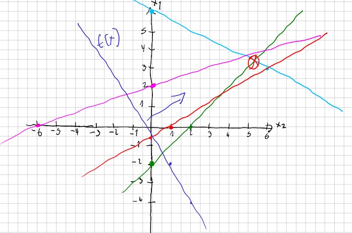
The solution is the line between (4,4) and (6, 0) with the maxiumum value of 12.
Problem 2
Determine for \(\beta \geq 2\), and the following sytem the possible solutions
$$ \begin{align} x_1 + x_2 - 2x_3 &= 1, \\ 2x_1 + 3x_2 - 5x_3 &= \beta, \\ 2x_2 - 5x_3 \leq 4 \end{align} $$For every \(\beta\) name its solution.
Solution
The system has a solution if and only if Phase 1 of the Simplex algorithm provides a solution. To achieve this, we introduce a variable \( x_5 \) for the third condition in order to bring the problem into normal form.
Then, we write our problem as a tableau
$$ \begin{array}{cccccc|c} x_1 & x_2 & x_3 & x_4 & x_5 & x_6 & b \\ \hline -3 & -4 & 7 & 0 & 0 & 0 & -1 - \beta \\ \hline \fbox{1} & 1 & -2 & 1 & 0 & 0 & 1 \\ 2 & 3 & -5 & 0 & 1 & 0 & \beta \\ 0 & 2 & -5 & 0 & 0 & 1 & 4 \end{array} $$The pivot element is in the first row and first column since it has the smallest pivot.
$$ \begin{array}{cccccc|c} x_1 & x_2 & x_3 & x_4 & x_5 & x_6 & b \\ \hline 0 & -1 & 1 & 3 & 0 & 0 & 2 - \beta \\ \hline 1 & 1 & -2 & 1 & 0 & 0 & 1 \\ 0 & 1 & -1 & -2 & 1 & 0 & \beta - 2 \\ 0 & 2 & -5 & 0 & 0 & 1 & 4 \end{array} $$We now look at the second column.
Case 1: \( \beta \geq 3 \) Then, the pivot is in the first row.
$$ \begin{array}{cccccc|c} x_1 & x_2 & x_3 & x_4 & x_5 & x_6 & b \\ \hline 0 & -1 & 1 & 3 & 0 & 0 & 2 - \beta \\ \hline 1 & \fbox{1} & -2 & 1 & 0 & 0 & 1 \\ 0 & 1 & -1 & -2 & 1 & 0 & \beta - 2 \\ 0 & 2 & -5 & 0 & 0 & 1 & 4 \end{array} $$Thus we get
$$ \begin{array}{cccccc|c} x_1 & x_2 & x_3 & x_4 & x_5 & x_6 & b \\ \hline 1 & 0 & -1 & 3 & 0 & 0 & 3 - \beta \\ \hline 1 & 1 & -2 & 1 & 0 & 0 & 1 \\ -1 & 0 & \fbox{1} & -3 & 1 & 0 & \beta - 3 \\ -2 & 0 & -1 & -2 & 0 & 1 & 2 \end{array} $$And hence
$$ \begin{array}{cccccc|c} x_1 & x_2 & x_3 & x_4 & x_5 & x_6 & b \\ \hline 0 & 0 & 0 & 1 & 1 & 0 & 0 \\ \hline -1 & 1 & 0 & -5 & 2 & 0 & 2\beta-5 \\ -1 & 0 & 1 & -3 & 1 & 0 & \beta - 3 \\ -3 & 0 & 0 & -5 & 1 & 1 & \beta - 1 \end{array} $$Thus, we are done and have found a solution with
\[ x^* = (0, 2\beta -5, \beta -3, 0). \]Case 2: \( 2 \leq \beta \leq 3 \) Then, the pivot is in the second row.
$$ \begin{array}{cccccc|c} x_1 & x_2 & x_3 & x_4 & x_5 & x_6 & b \\ \hline 0 & -1 & 1 & 3 & 0 & 0 & 2 - \beta \\ \hline 1 & 1 & -2 & 1 & 0 & 0 & 1 \\ 0 & \fbox{1} & -1 & -2 & 1 & 0 & \beta - 2 \\ 0 & 2 & -5 & 0 & 0 & 1 & 4 \end{array} $$Hence
$$ \begin{array}{cccccc|c} x_1 & x_2 & x_3 & x_4 & x_5 & x_6 & b \\ \hline 0 & 0 & 0 & 1 & 1 & 0 & 0 \\ \hline 1 & 0 & -1 & 3 & -1 & 0 & -\beta + 3 \\ 0 & \fbox{1} & -1 & -2 & 1 & 0 & \beta - 2 \\ 0 & 0 & -3 & 4 & -2 & 1 & -2\beta + 8 \end{array} $$And thus, we are done with the solution
\[ x^* = (-\beta + 3, \beta -2, 0). \]Problem 3
Given the function
$$ f(x, y) = ax^2 + by^2 - 4xy - 2x + 4y $$where \(a,b \in \mathbb{R}\) are parameters.
a) Determine all \(a,b\), so that f is convex.
b) For which \(a,b\) is \((1, 1)\) a local minima of \(f\).
Solution
a)
First, we determine the Hessian matrix of the function. The first derivative is
Thus, the Hessian matrix is
$$ \nabla^2 f = H_f = \begin{pmatrix} 2a & -4 \\ -4 & 2b \end{pmatrix} $$We determine whether the matrix is positive semidefinite and for which values by using the minors.
$$ det_1(H_f) = 2a $$$$ det_2(H_f) = 4ab - 12 $$That is, the matrix is semidefinite, and therefore the function \( f \) is convex, if and only if \( a \geq 0 \) and \( ab \geq 4 \).
b) For the minimum value, \(\nabla f = 0\) has to be true
$$ \begin{align} 2a - 6 =^! 0 \\ 2b =^! 0 \end{align} $$It follows that \( b = 0 \) and \( a = 3 \). Due to the condition \( ab \geq 4 \), the problem is not convex in this case.
For
this means that \( (1,1) \) is not a local minimum.
Problem 4
Let \(B\) be symmetric and positiv definit and \(A\) have full rank. Further, \(c\) is not in range of \(A^T\).
Given the problem
$$ \min \ c^Tx \ \ \text{under} \ \ x^TBx \leq 1, \ Ax = 0 $$a) Show that a minima \(x^*\) exists.
b) Proof, that \(AB^{-1}A^T\) is regular.
c) Show that \(\alpha\) exists with \(x^* = \alpha(Pc-B^{-1}c)\), where \(P = B^{-1}A^T(AB^{-1}A^T)^{-1}AB^{-1}\), is \(x^* = 0\)?
d) Determine \(\alpha\) and \(x^*\).
Solution
a)
The objective function is continuous. Furthermore, \( M \) is bounded because \( 0 < x^T B x \leq 1 \), and it is closed, thus compact. Since the objective function is continuous and the constraint set is compact, there exists a local solution (LSG).
b)
Since \( A \) has full rank, both \( A \) and \( A^T \) are bijective. Assume \( A B^{-1} A^T x = 0 \).
Let \( x A B^{-1} A^T x = (A^T x)^T B^{-1} (A^T x) = y^T B^{-1} y \). Then \( y^T B^{-1} y = 0 \) if and only if \( y = 0 \), because \( B^{-1} \) is positive definite.
It follows that \( x = 0 \). Thus, \( A B^{-1} A^T \) is bijective and, therefore, regular.
c)
The problem is convex because \( f(x) = c^T x \) and \( g(x) = x^T B x - 1 \) are convex, as \( B \) is symmetric and positive definite.
The Slater condition holds because:
- The rank of \( A \) is maximal.
- \( A x' = 0 \) and \( g(x') < 0 \), with \( x' = 0 \).
Thus, there is no duality gap, and a local solution (LSG) exists. We obtain this LSG using the Lagrange multiplier theorem, i.e.,
\[ L(x, u, v) = c^T x + u(x^T B x - 1) + v(Ax) \]For the LSG to hold, the following must be true:
\[ \begin{align} \nabla L = c + 2u B x + A^T v = 0 \\ u g(x) = u(x^T B x - 1) = 0 \end{align} \]In particular, \( x^* \neq 0 \), because otherwise, \( u = 0 \) must hold due to the second condition, but then we would have \( c = 0 \) from the first condition, which is impossible according to the assumption, as it would then lie in the image of \( A^T \).
Thus, it follows that \( x^* = - \frac{1}{2} u B^{-1} (c + A^T v) \). Substituting this into \( A x^* = 0 \), we obtain the desired form.
d)
Solving for \( \alpha \) gives the solution.
Problem 5
Given the function
$$ f(x) = x_1 + 2x_2 + 4x_3 $$and the set
$$ M = \{x_1 x_2 x_3 = 1, \ x_1, x_2, x_3 > 0\} $$a) Is M closed? Is M restricted?
b) Exist a global minima or maxima of f on M?
c) Determine all local and global minima and maxima of f on M.
Solution
a)
Let \((a_1), (a_2), (a_3)\) be any sequence in \(M\). Then, it holds that \(a_1 a_2 a_3 \to a^1 a^2 a^3 = 1\), and thus \(M\) is closed.
\(M\) is not bounded because \((t, 1/t, 0) \to (\infty, 0, 0)\).
b)
There is no maximum point because of the sequence \(a = (t, 1/t, 0) \in M\) and \(f(a) \to \infty\).
\(M\) is bounded from below because \(x_1, x_2, x_3 > 0\), and we can restrict ourselves to the set \(M = \{ f(x) < f(1, 1, 1) \}\). This set is closed and bounded, hence compact. Since \(f(x)\) is continuous, there exists a minimum point.
c)
The problem is differentiable because \(f(x)\) and \(g(x) = x_1 x_2 x_3 - 1\) are differentiable.
Let’s examine CQ1:
- \(\text{Rank}(h) = n\), which is satisfied since we do not have an \(h\) function.
- \(g(x) + u g'(x) < 0\), which is satisfied for \(x = 0\).
This means we can apply the Lagrange Multiplier Theorem. We first form the Lagrangian function:
\[ L(x, u, v) = x_1 + 2x_2 + 4x_3 + u(x_1 x_2 x_3 - 1) \]The LSG (local solution) is a KKT point, for which the following conditions hold:
\[ \begin{align} 0 &= 1 + u x_2 x_3 \\ 0 &= 2 + u x_1 x_3 \\ 0 &= 4 + u x_1 x_2 \end{align} \]Multiply the first equation by \(x_1\), the second by \(x_2\), and the third by \(x_3\), then we obtain \(x_1 x_2 x_3 = 1\).
\[ \begin{align} x_1 + u &= 0 \\ 2 x_2 + u &= 0 \\ 4 x_3 + u &= 0 \end{align} \]Thus, \(x^* = -u(1, 1/2, 1/4)\). The constraint \(x_1 x_2 x_3 = 1\) gives us \(u = -2\), and therefore \(f(x^*) = 6\).
Problem 6
Prove or disprove the following statement:
Every feasible optimization problem of the form
\[ \min f(x) \quad \text{subject to} \quad M = \{x \in X: g(x) \leq 0, h(x) = 0\} \]with \( X \subset \mathbb{R}^n \), \( f: X \to \mathbb{R} \), \( g: X \to \mathbb{R}^l \), and \( h: X \to \mathbb{R}^m \) has a solution, provided that
\[ \inf\{f(x): x \in M\} > -\infty. \]Solution
The given statement is incorrect. Consider the following counterexample:
\[ f(x) = |x|, \quad g(x) = x, \quad h(x) = x - 1 \]Then we have \( f(x) \geq 0 \). Furthermore, from \( h(x) = x - 1 = 0 \), we get \( x = 1 \), but the constraint \( g(x) \leq 0 \) requires \( x \leq 0 \), leading to a contradiction.
Another counterexample is:
\[ f(x) = e^x, \quad g(x) = 0, \quad h(x) = 0 \]Here, \( f(x) \geq 0 \) and has no solution because as \( x \to -\infty \), \( f(x) \to 0 \). This means we can always find a better \( x \), preventing the existence of an optimal solution.
Problem 7
A tire manufacturer produces two different types of tires made from different rubber compounds. For each tire set of type \( R_1 \) and \( R_2 \), different amounts of raw materials \( A \) and \( B \) are used, with a certain maximum capacity available per month. The sale of each tire set generates different profits, which, along with the other data, are listed in the following table:
\[ \begin{array}{c|ccc} \hline & R_1 & R_2 & Capacity \\ \hline \text{Raw material A (units per set)} & 1 & 2 & 32 \\ \text{Raw material B (units per set)} & 4 & 2 & 60 \\ \text{Profit (euros per set)} & 45 & 30 & \\ \hline \end{array} \]The tire manufacturer wants to maximize its profit. Formulate this linear optimization problem in standard form.
Solution
The optimization problem is formulated as:
\[ (P) \quad \max \ f(x) = 45 R_1 + 30 R_2 \]subject to:
\[ R_1 + 2 R_2 \leq 32, \quad 4 R_1 + 2 R_2 \leq 60, \quad R_1, R_2 \geq 0. \]In standard form, we convert the inequalities into equalities by introducing slack variables \( c_1 \) and \( c_2 \):
\[ (P) \quad \min \ f(x) = -45 R_1 - 30 R_2 \]subject to:
\[ R_1 + 2 R_2 + c_1 = 32, \]\[ 4 R_1 + 2 R_2 + c_2 = 60, \]\[ R_1, R_2, c_1, c_2 \geq 0. \]Problem 8
Solve the following linear optimization problem using the Simplex method and Bland’s rule:
\[ \max \quad x_1 + x_2 \]subject to:
\[ M = \{(x_1, x_2) \in \mathbb{R}^2 \mid x_1 + 2x_2 \geq 2, \quad 4x_1 + 4x_2 \leq 1\}. \]Solution
We first convert the problem into standard form by introducing unrestricted-sign variables:
\[ x_1 := x_1^+ - x_1^-, \quad x_2 := x_2^+ - x_2^- \]Additionally, we introduce slack variables \( x_3 \) and \( x_4 \). This gives us the following problem:
\[ (P) \quad \min f(x) = -x_1^+ + x_1^- - x_2^+ + x_2^- \]subject to:
\[ x_1^+ - x_1^- + 2x_2^+ - 2x_2^- - x_3 = 2, \]\[ 4x_1^+ - 4x_1^- + 4x_2^+ - 4x_2^- + x_4 = 1. \]Now, we construct the Simplex tableau:
\[ T_1: \quad \begin{array}{cccccc|c} -1 & 1 & -1 & 1 & 0 & 0 & \gamma \\ \hline 1 & -1 & 2 & -2 & -1 & 0 & 2 \\ 4 & -4 & 4 & -4 & 0 & 1 & 1 \end{array} \]Since the second-to-last column does not contain a unit vector, we begin Phase 1 of the Simplex algorithm, applied to this specific column.
$$ T_2: \ \ \begin{array}{ccccccc|c} -1 & 1 & -2 & 2 & 1 & 0 & 0 & -2 \\ \hline -1 & 1 & -1 & 1 & 0 & 0 & 0 & \gamma \\ \hline 1 & -1 & 2 & -2 & -1 & 0 & 1 & 2 \\ \fbox{4} & -4 & 4 & -4 & 0 & 1 & 0 & 1 \end{array} $$$$ T_3: \ \ \begin{array}{ccccccc|c} 0 & 0 & -1 & 1 & 1 & 1/4 & 0 & -7/4 \\ \hline 0 & 0 & 0 & 0 & 0 & 1/4 & 0 & \gamma + 1/4 \\ \hline 0 & 0 & 1 & -1 & -1 & -1/4 & 1 & 7/4 \\ 1 & -1 & \fbox{1} & -1 & 0 & 1/4 & 0 & 1/4 \end{array} $$$$ T_4: \ \ \begin{array}{ccccccc|c} 1 & -1 & 0 & 0 & 1 & 2/4 & 0 & -6/4 \\ \hline 0 & 0 & 0 & 0 & 0 & 1/4 & 0 & \gamma + 1/4 \\ \hline -1 & \fbox{1} & 0 & 0 & -1 & -2/4 & 1 & 6/4 \\ 1 & -1 & 1 & -1 & 0 & 1/4 & 0 & 1/4 \end{array} $$$$ T_5: \ \ \begin{array}{ccccccc|c} 0 & 0 & 0 & 0 & 0 & 0 & 1 & 0 \\ \hline 0 & 0 & 0 & 0 & 0 & 1/4 & 0 & \gamma + 1/4 \\ \hline -1 & 1 & 0 & 0 & -1 & -2/4 & 1 & 6/4 \\ 0 & 0 & 1 & -1 & -1 & -1/4 & 1 & 7/4 \end{array} $$Phase 1 of the Simplex algorithm is now complete, and we can proceed to Phase 2. However, as we can see, Phase 2 is already finished since all entries in the corresponding row are non-negative.
Thus, our solution is:
\[ x_1^+ = 0, \quad x_1^- = \frac{3}{2}, \quad x_2^+ = \frac{7}{4}, \quad x_2^- = 0, \quad x_3 = 0, \quad x_4 = 0. \]This means our final solution is:
\[ x^* = \left(-\frac{3}{2}, \frac{7}{4} \right) \]with an optimal function value:
\[ f(x^*) = 0. \]Problem 9
Consider the following optimization problem:
\[ (P) \quad \min \left( x_1 + e^{x_2} \right) \]subject to:
\[ 3x_1 - 2e^{x_2} \geq 10 \quad \text{and} \quad x_2 \geq 0. \](a) Prove that this is a convex optimization problem.
(b) Show that the Slater condition is satisfied for (P).
(c) Formulate the dual problem (D) of (P). Explicitly give the function in (D) that appears as:
\[ F(u, v) = \inf_{x \in \mathbb{R}^2} L(x, u, v). \](d) Solve (D).
Solution a)
First, let’s consider the objective function \( f \) and form its Hessian matrix \( H_f \):
\[ \nabla f(x) = (1, e^{x_2}), \quad \nabla^2 f = H_f = \begin{pmatrix} 0 & 0 \\ 0 & e^{x_2} \end{pmatrix} \]Next, we look at the minors to determine definiteness:
\[ \text{det}_1(H_f) = 0, \quad \text{det}_2(H_f) = 0 \]Since all minors are 0, our function is semi-positive definite, and thus convex.
Next, we examine the constraints \( g_1(x) = -3 x_1 + 2 e^{x_2} + 10 \) and \( g_2(x) = -x_2 \). We compute their derivatives:
\[ \nabla g_1 = (-3, 2e^{x_2}), \quad \nabla g_2 = (0, 0), \]\[ \nabla^2 g_1 = H_{g_1} = \begin{pmatrix} 0 & 0 \\ 0 & 2e^{x_2} \end{pmatrix}, \quad \nabla^2 g_2 = H_{g_2} = \begin{pmatrix} 0 & 0 \\ 0 & 0 \end{pmatrix} \]Now, we check their minors:
\[ \text{det}_1(H_{g_1}) = 0, \quad \text{det}_2(H_{g_1}) = 0, \quad \text{det}_1(H_{g_2}) = 0, \quad \text{det}_2(H_{g_2}) = 0 \]Since all minors are 0, the functions are semi-positive definite and thus convex.
Since both the objective function and the constraints are convex, our problem is convex.
Solution b)
The Slater condition is satisfied because we don’t have a constraint of the form \( Ax = b \). Therefore, the first condition is fulfilled. Additionally, for the point \( (x_1, x_2) = (10, 1) \), we have:
\[ g_1(10, 1) = -3(10) + 2e^{1} + 10 < 0, \quad g_2(10, 1) = -1 < 0. \]Since both inequality constraints are strictly satisfied at \( (10, 1) \), the Slater condition is fulfilled.
Solution c)
First, we set up the Lagrangian function:
\[ L(x, u, v) = x_1 + e^{x_2} + u_1 (-3x_1 + 2e^{x_2} + 10) - u_2 x_2 \]Now, we seek \( F(u) \), which involves finding where \( L \) attains its infimum. To do this, we solve for the derivatives:
\[ (1) \quad 0 = \nabla_{x_1} L = 1 - 3 u_1 x_1 \]\[ (2) \quad 0 = \nabla_{x_2} L = e^{x_2} + 2 u_1 e^{x_2} - u_2 \]From (1), we get \( \frac{1}{3} u_1 = x_1 \). From (2), we get:
\[ u_2 = e^{x_2} + 2 u_1 e^{x_2} \]\[ \iff u_2 = e^{x_2} (1 + 2 u_1) \]\[ \iff \ln(u_2) = \ln(e^{x_2} (1 + 2 u_1)) \]\[ \iff \ln(u_2) = \ln(e^{x_2}) + \ln(1 + 2 u_1) \]\[ \iff \ln(u_2) = x_2 + \ln(1 + 2 u_1) \]\[ \iff x_2 = \ln\left( \frac{u_2}{1 + 2 u_1} \right) \]Now, we substitute our result into the Lagrangian function:
\[ F(x, u) = \frac{1}{3} u_1 + e^{\ln\left( \frac{u_2}{1 + 2 u_1} \right)} + u_1 \left( -3 \cdot \frac{1}{3} u_1 + 2 e^{\ln\left( \frac{u_2}{1 + 2 u_1} \right)} + 10 \right) - u_2 \ln\left( u_2 (1 + 2 u_1) \right) \]\[ = \frac{1}{3} u_1 + \frac{u_2}{1 + 2 u_1} + u_1 \left( -u_1 + 2 \cdot \frac{u_2}{1 + 2 u_1} + 10 \right) - u_2 \ln\left( \frac{u_2}{1 + 2 u_1} \right) \]\[ = \frac{1}{3} u_1 + \frac{u_2}{1 + 2 u_1} - u_1^2 + 2 u_1 \frac{u_2}{1 + 2 u_1} + 10 u_1 - u_2 \ln\left( \frac{u_2}{1 + 2 u_1} \right) \]\[ = \frac{1}{3} u_1 + u_2 - u_1^2 + 10 u_1 - u_2 \ln\left( \frac{u_2}{1 + 2 u_1} \right) \]\[ = u_2 + \frac{1}{3} u_1 - u_1^2 - u_2 \ln\left( \frac{u_2}{1 + 2 u_1} \right) + 10 u_1 \]Furthermore, we have the restriction that \( F(u) \) must be greater than \(-\infty\), meaning we need to check for which \( u_i \) this condition is satisfied.
It must be that \( u_2 \geq 0 \), because otherwise, as \( u_2 \to -\infty \), we would also have \( F(u) \to -\infty \). Similarly, \( u_1 = \frac{1}{3} \) must hold. Thus, we obtain:
\[ F(u) = u_2 - u_2 \ln\left( \frac{u_2}{1 + 2/3} \right) + \frac{10}{3} \]Thus, the dual problem is:
\[ (D) \quad \max F(u) \quad \text{subject to} \quad u_2 \geq 0 \]Solution d)
Since the Slater condition is satisfied, the strong duality theorem holds, and therefore \( \max(F) = \min(f) \).
Now, we examine the derivative of \( F(u) \):
\[ F'(u_2) = 1 - \ln\left( \frac{u_2}{1 + 2/3} \right) - u_2 \cdot \frac{1}{u_2 \ln\left( \frac{u_2}{1 + 2/3} \right)} = -\ln\left( \frac{3 u_2}{5} \right) \]Next, we solve:
\[ F'(u_2) = 0 \quad \iff \quad 1 = \frac{3 u_2}{5} \quad \iff \quad u_2 = \frac{5}{3} \]Thus, the maximum of \( F \) occurs at the point \( u_1 = \frac{1}{3}, u_2 = \frac{5}{3} \), with \( F(u_2) = 5 \).
Problem 10
Look at the following optimization problem
$$ (P) \quad \min \ (x_{1}-1)^{2}-x_{2}^{2}+x_{3}^{2}-4x_{3} $$subject to
$$ x_{1}+x_{2}-x_{3}=0 $$$$ x_{2}+x_{3}^{2}=0 $$(a) Determine all KKT points of (P).
(b) Using the necessary second-order optimality condition, show that the function f does not have a local minimum at the point (0,-1,-1).
Solution a)
The CQ1 condition is satisfied, because we don’t have \( Ax = b \), which satisfies the first condition. Additionally, with \( z = 0 \) and \( h'(x) z = 0 \), the second condition is fulfilled.
Now, we formulate the Lagrangian function:
\[ L(x, v) = (x_1 - 1)^2 - x_2^2 + x_3^2 - 4x_3 + v_1 (x_1 + x_2 - x_3) + v_2 (x_2 + x_3^2) \]For the KKT points, we have the following conditions:
\[ (1) \quad 0 = \nabla_{x_1} L = 2(x_1 - 1) + v_1 \]\[ (2) \quad 0 = \nabla_{x_2} L = -2x_2 + v_1 + v_2 \]\[ (3) \quad 0 = \nabla_{x_3} L = 2x_3 - 4 - v_1 + 2v_2x_3 \]\[ (4) \quad 0 = h_1 = x_1 + x_2 - x_3 \]\[ (5) \quad 0 = h_2 = x_2 + x_3^2 \]From (1), we get:
\[ v_1 = -2(x_1 - 1) \]Next, from (2), by substitution, we get:
\[ v_2 = 2x_2 + 2(x_1 - 1) \]Substituting into (3), we get:
\[ 0 = 2x_3 - 4 + 2(x_1 - 1) + 2x_3 (2x_2 + 2(x_1 - 1)) \]\[ \iff 2 = x_3 + (x_1 - 1) + x_3(2x_2 + 2x_1 - 2) \]\[ \iff 3 = x_3 + x_1 + 2x_2 x_3 + 2x_1 x_3 - 2x_3 \]\[ \iff 3 = x_1 + 2x_2 x_3 + 2x_1 x_3 - x_3 \]In the above equation, we can substitute (4) and (5):
\[ 3 = (x_3 + x_3^2) + 2(-x_3^2) x_3 + 2(x_3 + x_3^2) x_3 - x_3 \]\[ \iff 3 = x_3 + x_3^2 - 2x_3^3 + 2x_3^2 + 2x_3^3 - x_3 \]\[ \iff 3 = 3x_3^2 \]Thus, we find the solution \( x_3 \in \{1, -1\} \). With (5) and then (4), we obtain the KKT points \( (2, -1, 1, -2, 0) \) and \( (0, -1, -1, 2, -4) \).
Solution b)
According to the necessary second-order optimization condition, \( f \) does not have a local minimum at a point if the second derivative at this point is not positive definite.
The Hessian matrix is:
\[ \nabla^2 f = H_f = \begin{pmatrix} 2 & 0 & 0 \\ 0 & -2 & 0 \\ 0 & 0 & 2 + v_2 \end{pmatrix} \]Now, we examine the principal minors to check for definiteness:
\[ \text{det}_1(H_f) = 2 > 0, \quad \text{det}_2(H_f) = 2 \cdot (-2) = -4 < 0 \]Since the second minor is negative, \( H_f \) is not positive definite, and thus the point is not a local minimum.
Problem 11
Prove the following statement:
If the minimum of the linear optimization problem
\[ \min \ f(x) \text{ on } \{x \in \mathbb{R}^{n}_{\geq 0} \mid Ax = b\} \]is attained at more than one vertex, then it is attained on the convex hull of these vertices.
Solution
Let \( E \) be the set of vertices that are the minima, and let \( x_i \) represent these minima.
The convex hull of this set is given by:
$$ \text{conv}(E) = \left\{ \sum \lambda_i x_i : x_i \in E, \lambda_i \geq 0, \sum \lambda_i = 1 \right\} $$Let \( x^* \in \text{conv}(E) \). Then:
$$ f(x^*) = f\left( \sum \lambda_i x_i \right) = \sum \lambda_i f(x_i) = f(x_1) \sum \lambda_i = f(x_1) $$Thus, \( x^* \) is a minimum of \( f \).
Problem 12
Let \( A \in \mathbb{R}^{m \times n} \), \( b \in \mathbb{R}^m \). Prove the following Gale’s Alternative Theorem: Exactly one of the following two statements is true:
$$ \text{(I)} \quad Ax = b \text{ has a solution } x \in \mathbb{R}^n $$or
$$ \text{(II)} \quad A^T y = 0, \quad y \geq 0, \quad b^T y < 0 \text{ has a solution } y \in \mathbb{R}^m $$Solution
We first introduce the sign-restricted variables \(x^{+}, x^{-} \geq 0\) and write \(x = x^{+} - x^{-}\). By further introducing the slack variable \(z \in \mathbb{R}^{n_2}\), we find that the system \(Ax \leq b\) is equivalent to the linear system of equations:
$$ \begin{pmatrix} A & -A & I \\ \end{pmatrix} \begin{pmatrix} x^{+} \\ x^{-} \\ z \end{pmatrix} = b \tag{5} $$Applying Farkas’ Lemma to (5) now states that either (and exclusively) the system (5) or the system
$$ \begin{pmatrix} A^{T} \\ -A^{T} \\ I \end{pmatrix} y \leq 0 \text{ and } b^{T}y > 0 \tag{6} $$has a solution. The system (6) is, in turn, equivalent to the system
$$ \begin{aligned} A^{T}y &= 0 \\ y &\leq 0 \\ b^{T}y &> 0. \end{aligned} $$With this the theorem has been shown.
Problem 13
Consider the linear program in standard form with \(A \in \mathbb{R}^{K \times N}\), \(b \in \mathbb{R}^K\), and \(c \in \mathbb{R}^N\):
$$ (P) \quad \min c^T x \ \ \text{over} $$$$ M = \{x \in \mathbb{R}^N : Ax = b, x \ge 0\} $$(a) Formulate the dual problem (D) to (P).
(b) Formulate Farkas’ Lemma for \(A \in \mathbb{R}^{K \times N}\) and \(b \in \mathbb{R}^K\).
Given the optimization problem:
$$ (P) \quad \min \ x_1 + x_3 \ \ \text{subject to:} $$$$ x_1 \ge 1 $$$$ x_2 \ge 0 $$$$ x_1 - x_2 - x_3 = 1 $$$$ x_1 + x_2 + x_3 = 1 $$$$ x_1 + x_2 - x_3 = 2 $$(c) Convert the optimization problem (P) into standard form. Explicitly provide \(A\), \(b\), and \(c\).
(d) Show that the dual problem to (P) is feasible.
Solution a)
The dual problem to \((P)\) is given by
\[ (D) \quad \max \ b^T y \quad \text{subject to} \quad N = \{A^T y \leq c\} \]Solution b)
Farkas’ Lemma states that exactly one of the following statements is always true:
- \( Ax \leq b, \quad x \geq 0 \)
- \( A^T y \leq 0, \quad b^T y > 0 \)
Solution c)
To bring the problem into standard form, we introduce sign-restrictive variables \( x_3 = x_3^+ - x_3^- \) with \( x_3^+, x_3^- \geq 0 \).
Additionally, we introduce a slack variable \( x_4 \).
The problem then becomes:
\[ (P) \quad \min x_1 + x_3^+ - x_3^- \quad \text{subject to:} \]\[ x_1 + x_2 + x_3^+ - x_3^- = 1 \]\[ x_1 - x_2 - x_3^+ + x_3^- = 2 \]\[ x_1 + x_2 - x_3^+ - x_3^- = 1 \]\[ x_1 - x_4 = 1 \]\[ x_1, x_2, x_3^+, x_3^-, x_4 \geq 0 \]Rewriting in matrix form:
\[ (P) \quad \min c^T x \quad \text{subject to } x \in M \]where
\[ M = \{x \in \mathbb{R}^5 : Ax = b, x \geq 0\} \]with
\[ c = (1, 0, 1, -1, 0) \]\[ b = (1, 2, 1, 1) \]\[ A = \begin{pmatrix} 1 & 1 & 1 & -1 & 0 \\ 1 & -1 & -1 & 1 & 0 \\ 1 & 1 & -1 & -1 & 0 \\ 1 & 0 & 0 & 0 & -1 \end{pmatrix} \]Solution d)
Choose the point \( x = (1, 1/2, -1/2, 0) \) (this point can be found using Gaussian elimination). Then, \( x \in M \), and thus the set is feasible.Problem 14
a) State the Projection Theorem for Convex Sets.
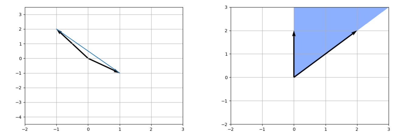
b) Sketch the following sets in \( \mathbb{R}^2 \):
$$ K = \text{conv} \left\{ \begin{pmatrix} -1 \\ 2 \end{pmatrix}, \begin{pmatrix} 1 \\ -1 \end{pmatrix} \right\}, \quad V = \text{cone} \left( \begin{pmatrix} 0 \\ 2 \end{pmatrix}, \begin{pmatrix} 2 \\ 2 \end{pmatrix} \right) $$c) Formulate the Nash Equilibrium for a Two-Person Matrix Game. Define the strategy sets for player \( P_1 \) and player \( P_2 \), as well as the expected average payoff for a payoff matrix \( A \in \mathbb{R}^{K \times N} \). When is the matrix game considered fair?
Solution a)
Projection Theorem
Let \(\emptyset \neq M \subset \mathbb{R}^n\) be a closed and convex set. For any \(x \in \mathbb{R}^n\), there exists a unique \(x^* \in M\) such that
\[ \|x - x^*\| \leq \|x - z\| \quad \forall z \in M \]\[ (x - x^*)^T (z - x^*) \leq 0 \quad \forall z \in M. \]This means that \(x^*\) is the closest point in \(M\) to \(x\), and the second condition ensures that the vector \(x - x^*\) is orthogonal to the set \(M\) in a generalized sense.
Solution b)
Solution c)
The strategy sets for players \( P_1 \) and \( P_2 \) in a two-player matrix game are given as:
\[ M_1 = \left\{ x \in \mathbb{R}^n : e^T x = 1, x \geq 0 \right\} \]and
\[ M_2 = \left\{ y \in \mathbb{R}^n : e^T y = 1, y \geq 0 \right\} \]The expected payoff for the matrix game with payoff matrix \( A \) is given by:
\[ y^T A x \]A matrix game with players \( P_1 \) and \( P_2 \) is in Nash equilibrium if and only if the following condition holds:
\[ \max_{x \in M_1} \min_{y \in M_2} y^T A x = \min_{y \in M_2} \max_{x \in M_1} y^T A x \]A matrix game is fair if the expected payoff is 0:
\[ y^T A x = 0 \]This means that, on average, neither player has an advantage.
Problem 15
a) Sketch the polar cone to the set of all \( x \in \mathbb{R}^2 \) with the following conditions:
\[ 2x_2 \le 2, \quad 2x_1 - x_2 \le 0, \quad x_2 \ge 0, \quad 2x_1 \ge x_2 \]and the set itself.
b) Show that \( (-M)^\circ = -(M^\circ) \).
c) Let \( M_1 \subset M_2 \). Show that \( M_2^\circ \subset M_1^\circ \).
d) Show that the polar cone is a convex set.
e) Let \( C \) be a cone. Show that for the convex projection \( P_C(x) = 0 \), this holds if and only if \( x \in C^\circ \).
f) Let \( V \subset \mathbb{R}^N \) be a linear subspace. Show that the corresponding polar cone to \( V \) is given by:
\[ V^\circ = V^\perp = \{x \in \mathbb{R}^N : v^T x = 0 \text{ for all } v \in V\} \]Solution a)
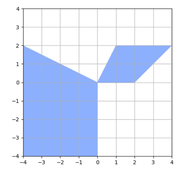
On the left is the polar cone and on the right the original set.
Solution b)
$$ \begin{align*} (-M)^\circ &= \{ x \in \mathbb{R}^n : y^T x \leq 0, \forall y \in (-M) \} \\ &= \{ x \in \mathbb{R}^n : -y^T x \leq 0, \forall y \in M \} \\ &= -\{ x \in \mathbb{R}^n : y^T x \leq 0, \forall y \in M \} \\ &= -(M)^\circ \end{align*} $$Solution c)
Let \( M_1 \subset M_2 \). For \( x_2 \in M_2^\circ \), it holds that \( y_2^T x_2 \leq 0 \) for all \( y_2 \in M_2 \). In particular, this also holds for \( y_1 \in M_1 \subset M_2 \). Therefore, \( x_2 \in M_1^\circ \) and \( M_2^\circ \subset M_1^\circ \).Solution d)
Let \( \lambda \in (0,1) \) and \( x_1, x_2 \in M^\circ \) arbitrarily fixed. Then it holds that
\[ y^T (\lambda x_1 + (1 - \lambda) x_2) = \lambda y^T x_1 + (1 - \lambda) y^T x_2 \leq 0 \]Thus, \( M^\circ \) is convex.
Solution e)
Since \( 0 \in C \) and the convex projection is unique, it follows that
\[ x^* = P_C(x) = 0 \iff (x - 0)^T(y - 0) \leq 0, \ \forall y \in M \]Thus, for all \( y \in M \), it holds that \( x^T y \leq 0 \), so \( x \in C^\circ \).
Solution f)
$$ \begin{align} V^\circ &= \{ x \in \mathbb{R}^n : v^T x \leq 0, \ \forall v \in M \} \\ &= \{ x \in \mathbb{R}^n : v^T x \leq 0, \ -v^T x \leq 0, \ \forall v \in M \} \\ &= \{ x \in \mathbb{R}^n : v^T x \leq 0, \ v^T x \geq 0, \ \forall v \in M \} \\ &= \{ x \in \mathbb{R}^n : v^T x = 0, \ \forall v \in M \} \end{align} $$Problem 16
Given the linear program:
$$ (P) \quad \min \ x_1 - 4x_2 - 2x_3 \ \ \text{subject to} $$\[ x_1 + x_3 \le 2 \]\[ x_1 + x_2 \le 4 \]\[ x_2 + x_3 \le 8 \]\[ x \geq 0 \]a) Formulate the pivot rule according to Bland.
b) Solve the linear program using the Simplex method.
Solution a)
Pivot rule according to Bland:
- First, find the first column whose first entry is negative, i.e., \( i := \min\{ i : c_i \leq 0 \} \)
- If all \( a_{ij} < 0 \), then \( \inf(P) = -\infty \)
- Then, find the row whose quotient with the \( b \)-vector is the smallest, i.e., \( j := \min\{ j : b_j / a_{ij} \} \)
- Our pivot is then \( a_{ij} \)
Solution b)
First, we bring our problem into standard form by introducing slack variables \( s_1, s_2, s_3 \) for each constraint. We can directly start with Phase 2 of the Simplex algorithm and thus obtain the following tableau:
\[ T_1 : \ \ \begin{array}{cccccc|c} 1 & -4 & -2 & 0 & 0 & 0 & \gamma \\ \hline 1 & 0 & 1 & 1 & 0 & 0 & 2 \\ 1 & \fbox{1} & 0 & 0 & 1 & 0 & 4 \\ 0 & 1 & 1 & 0 & 0 & 0 & 8 \\ \end{array} \]\[ T_2 : \ \ \begin{array}{cccccc|c} 5 & 0 & -2 & 0 & 4 & 0 & \gamma + 16 \\ \hline 1 & 0 & \fbox{1} & 1 & 0 & 0 & 2 \\ 1 & 1 & 0 & 0 & 1 & 0 & 4 \\ -1 & 0 & 1 & 0 & -1 & 0 & 4 \\ \end{array} \]\[ T_3 : \ \ \begin{array}{cccccc|c} 7 & 0 & 0 & 2 & 4 & 0 & \gamma + 20 \\ \hline 1 & 0 & 1 & 1 & 0 & 0 & 2 \\ 1 & 1 & 0 & 0 & 1 & 0 & 4 \\ -2 & 0 & 0 & -1 & -1 & 0 & 2 \\ \end{array} \]Thus, we are done and have the optimal solution \( x^* = (0, 4, 2) \) with \( f(x^*) = -20 \).
Problem 17
Given the optimization problem in \( \mathbb{R}^2 \):
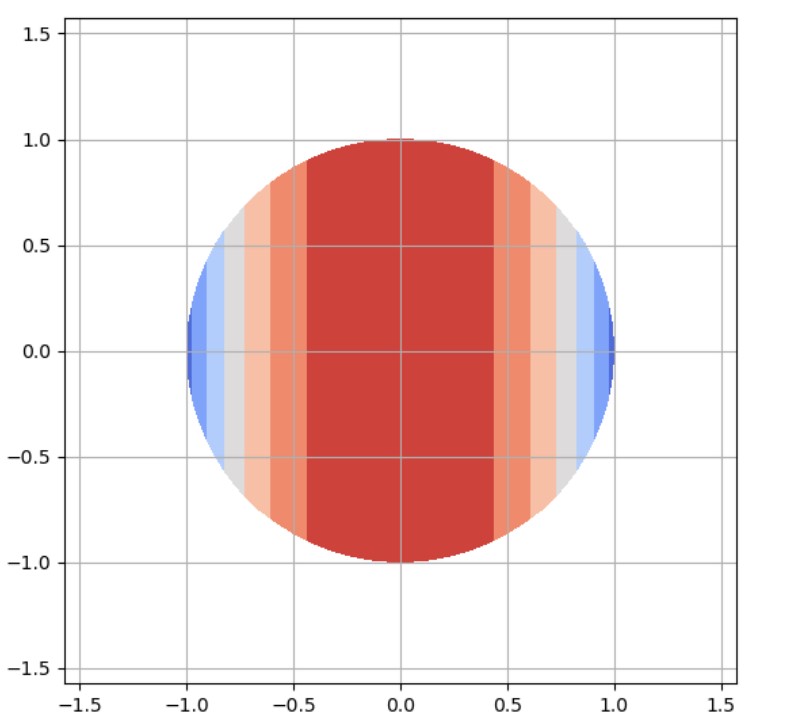
$$ (P) \quad \min \ f(x) = -\exp\left(-\frac{x_1^2}{2}\right) \ \ \text{subject to} \ \ x_1^2 + x_2^2 \le 1. $$a) Sketch the feasible set.
b) Determine all the KKT points of the problem (P).
c) Show that the KKT points satisfy the (CQ2) condition.
d) Show that the KKT points satisfy the second-order necessary condition.
Solution a)
Solution b)
We first set up the Lagrange function:
$$ L(x, u) = -\exp\left(-\frac{x_1^2}{2}\right) + u(x_1^2 + x_2^2 - 1) $$We then obtain the following conditions for the KKT points:
\[ \begin{aligned} 0 &= \nabla_{x_1} f = x_1 \exp\left(-\frac{x_1^2}{2}\right) + 2u x_1 \quad &(1) \\ 0 &= \nabla_{x_2} f = 2u x_2 \quad &(2) \\ 0 &= u g = u(x_1^2 + x_2^2 - 1) \quad &(3) \\ 0 &\geq g = x_1^2 + x_2^2 - 1 \quad &(4) \end{aligned} \]Case 1 (u = 0): Substituting into (1), we get:
$$ 0 = x_1 \exp\left(-\frac{x_1^2}{2}\right) \implies x_1 = 0 $$From (4), we then have \(x_2^2 \leq 1\), i.e., \(x_2 \in [-1, 1]\), and thus we obtain the KKT points \(((0, x_2), 0)\).
Case 2 \(u > 0\): From (2), we obtain \(x_2 = 0\), and from (3) we get \(1 = x_1^2\), so \(x_1 = \pm 1\). Substituting \( \pm 1 \) into (1):
$$ x_1 \exp\left(-\frac{1}{2}\right) + 2u = 0 \implies u = -\frac{1}{2} \exp\left(-\frac{1}{2}\right) $$This leads to a contradiction because \(\exp\left(-\frac{1}{2}\right)\) is not negative and cannot equal \(-\infty\). Therefore, there are no KKT points in this case.
Solution c)
We calculate the derivative of \(g\):
$$ \nabla g = (2x_1, 2x_2) $$We substitute the KKT points we found:
$$ \nabla g((0, x_2)) = (0, 2x_2) \quad \text{with} \quad x_2 \in [-1, 1] $$This is linearly independent for all points and thus CQ2 is satisfied.
Solution d)
To check if the second-order necessary condition is satisfied, we need to verify if \(f\) is positive definite.
That is, we first calculate the Hessian matrix of \(f\):
$$ \nabla^2 f = H_f = \begin{pmatrix} \exp\left(-\frac{x_1^2}{2}\right)(1 - x_1^2) & 0 \\ 0 & 2u \end{pmatrix} $$We now look at the minors to check definiteness:
$$ \det_1(H_f) = \exp\left(-\frac{x_1^2}{2}\right)(1 - x_1^2), \quad \det_2(H_f) = \exp\left(-\frac{x_1^2}{2}\right)(1 - x_1^2) \cdot 2u $$These are positive for the point \(((0, x_2), 0)\) with \(x_2 \in [-1, 1]\).
Problem 18
Let \( \emptyset \neq M \subset \mathbb{R}^N \) be a convex set, and \( f: \mathbb{R}^N \to \mathbb{R} \) be a convex function. The optimization problem is given by:
$$ (P) \quad \min f(x) \ \ \text{subject to} \ \ x \in M \ $$a) Show that the solution set of (P):
$$ M^* := \{ x \in M : f(x) \leq f(y), \forall y \in M \} $$is convex.
b) Let \( \emptyset \neq M \subset \mathbb{R}^N \) now be a polytope. Show that \( f \) attains its maximum on \( V = \{ x \in M : x \text{ is a vertex of } M \} \).
Hint: You can use the fact that for \( y^k \in M, k = 1, \dots, K \),
$$ f\left(\sum_{k=1}^K \lambda_k y^k\right) \leq \sum_{k=1}^K \lambda_k f(y^k), \quad \lambda_k \geq 0, \quad \sum_{k=1}^K \lambda_k = 1. $$Now, for \( g: \mathbb{R}^N \to \mathbb{R}^P \) convex, and \( A \in \mathbb{R}^{K \times N} \) and \( b \in \mathbb{R}^K \), the set \( M \) is given by:
$$ M = \{ x \in \mathbb{R}^N : g(x) \leq 0, Ax = b \}. $$c) State the Slater conditions for convex optimization problems.
d) Formulate the dual problem (D) for the convex optimization problem (P) on \( M \), and state the strong duality theorem.
Solution a)
Let \( x_1, x_2 \in M^* \) be two solutions and let \( \lambda \in (0,1) \). Since \( x_1 \) and \( x_2 \) are both minima, we have \( f(x_1) = f(x_2) \), and thus:
\[ \begin{aligned} f(\lambda x_1 + (1 - \lambda) x_2) &\leq \lambda f(x_1) + (1 - \lambda) f(x_2) \\ &= \lambda f(x_1) + (1 - \lambda) f(x_1) \\ &= f(x_1) \leq f(y), \quad \forall y \in M. \end{aligned} \]Therefore, \( M^* \) is convex.
Solution b)
Since \( M \) is a polytope, it has a finite number of vertices. Let \( c^* = \arg\max_{c \in V} f(c) \), and suppose \( \sum \lambda_k = 1 \). Then, for every \( x \in M \), we have:
\[ \begin{aligned} f(c^*) &= \sum \lambda_k f(c^*) \\ &\geq \sum \lambda_k f(c^k) \\ &\geq f\left(\sum \lambda_k c^k\right) \\ &= f(x). \end{aligned} \]Thus, the global maximum is attained at \( c^* \).
Solution c)
The Slater condition states:
- \( \operatorname{rank}(A) = n \leq m \).
- There exists \( x' \in \mathbb{R}^n \) such that \( g(x') \leq 0 \) and \( Ax' = b \).
Solution d)
The dual problem is given by
$$ (D) \quad \max \ f^*(u, v) \quad \text{subject to} \quad M^* = \{(u,v) \in \mathbb{R}^p \times \mathbb{R}^K : u \geq 0, f^*(u, v) > - \infty\} $$where
$$ f^*(u, v) = \inf_x L(x, u, v) = \inf_x \left[ f(x) + u^T g(x) + v^T (Ax - b) \right]. $$If both (P) and (D) are feasible and the Slater condition holds, then:
- (P) is solvable \( \iff \) (D) is solvable.
- Complementary slackness holds: \( u g(x^*) = 0 \).
- The strong duality property holds:
Problem 19
Prove or disprove: If \( f: \mathbb{R}^n \to \mathbb{R} \) is strictly convex and \( M \subset \mathbb{R}^n \) is convex and closed, so has problem
\[ (P) \quad \min_{x \in M} f(x) \]a solution.
Solution
There is a theorem stating that an optimization problem has a solution if \( f \) is continuous and \( M \) is closed and bounded.
Since \( f \) is convex, it is also continuous. However, boundedness is missing, meaning there must exist a constant \( c \) such that
\[ \forall x \in M: |x| \leq c. \]For example, \( [1,1] \) is bounded, but \( (-\infty, 0] \) is not. Since \( M \) is not necessarily bounded, the theorem does not apply.
Counterexample:
Let \( f(x) = e^x \) and \( M = \mathbb{R} \). Then, there is no solution because we can always find an \( x \) where \( f(x) \) is smaller.
Problem 20
A brewery can produce beers in three different flavors by mixing two types of hops. The table below specifies how many units (ME) of each hop type are required to produce one unit of each beer type. Additionally, the available quantity of each hop type and the profit per unit of each beer type are given. A minimum of 20 units of beer must be produced in total.
\[ \begin{array}{|c|cc|c|} \hline & \text{ME Hops 1} & \text{ME Hops 2} & \text{Profit per ME} \\ \hline \text{Beer 1} & 1 & 2 & 12 \\ \text{Beer 2} & 3 & 1 & 20 \\ \text{Beer 3} & 1 & 3 & 18 \\ \hline \text{Available (ME)} & 30 & 40 & \\ \hline \end{array} \]The brewery aims to maximize its profit. Formulate the problem as a linear optimization problem in standard form.
Solution
We have the standard form:
\[ (P) \quad \min c^T x \quad \text{subject to } x \in M \]with
\[ c = (-12, -20, -18, 0, 0, 0), \quad b = (30, 40, 20), \]\[ A = \begin{pmatrix} 1 & 3 & 1 & 1 & 0 & 0 \\ 2 & 1 & 3 & 0 & 1 & 0 \\ 1 & 1 & 1 & 0 & 0 & -1 \\ \end{pmatrix} \]where \( x_4, x_5, x_6 \) are slack variables.
Problem 21
We want to solve the following linear optimization problem using the Simplex Method:
\[ \text{Maximize} \quad x_2 - x_1 \quad \text{subject to} \quad x \in M = \{x \in \mathbb{R}^2 : 2x_1 + x_2 \geq 2, x_1 \geq 0, x_1 + x_2 \leq 3\}. \]Solution
First, we convert the problem into standard form. To do this, we introduce sign-independent variables, \( x_2 = x_2^+ - x_2^- \), and slack variables \( s_1, s_2 \).
Thus, we get the tableau.
$$ T_1 : \ \ \begin{array}{ccccc|c} 1 & -1 & 1 & 0 & 0 & \gamma \\ \hline 2 & 1 & -1 & -1 & 0 & 2 \\ 1 & 1 & -1 & 0 & 1 & 3 \end{array} $$We cannot immediately read off a basic solution because the second-to-last column is not a unit vector, so we start with phase 1 of the simplex algorithm applied to the first row.
$$ T_2 : \ \ \begin{array}{cccccc|c} -2 & -1 & 1 & 1 & 0 & 0 & -2 \\ \hline 1 & -1 & 1 & 0 & 0 & 0 & \gamma \\ \hline \fbox{2} & 1 & -1 & -1 & 0 & 1 & 2 \\ 1 & 1 & -1 & 0 & 1 & 0 & 3 \end{array} $$$$ T_3 : \ \ \begin{array}{cccccc|c} 0 & 0 & 0 & 0 & 0 & 1 & 0 \\ \hline 0 & -3/2 & 3/2 & 1/2 & 0 & -1/2 & \gamma - 1 \\ \hline 1 & 1/2 & -1/2 & -1/2 & 0 & 1/2 & 1 \\ 0 & 1/2 & -1/2 & 1/2 & 1 & -1/2 & 2 \end{array} $$Since the first row is positive, we are finished with phase 1 and can move on to phase 2 of the simplex algorithm.
$$ T_4 : \ \ \begin{array}{ccccc|c} 0 & -3/2 & 3/2 & 1/2 & 0 & \gamma - 1 \\ \hline 1 & \fbox{1/2} & -1/2 & -1/2 & 0 & 1 \\ 0 & 1/2 & -1/2 & 1/2 & 1 & 2 \end{array} $$$$ T_5 : \ \ \begin{array}{ccccc|c} 3 & 0 & 0 & -1 & 0 & \gamma + 2 \\ \hline 2 & 1 & -1 & -1 & 0 & 2 \\ -1 & 0 & 0 & \fbox{1} & 1 & 1 \end{array} $$$$ T_6 : \ \ \begin{array}{ccccc|c} 2 & 0 & 0 & 0 & 1 & \gamma + 3 \\ \hline 1 & 1 & -1 & 0 & 1 & 3 \\ -1 & 0 & 0 & 1 & 1 & 1 \end{array} $$Thus, we are finished with phase 2 of the simplex algorithm, and the solution is \( x^* = (0, 3) \) with \( f(x^*) = 3 \).
Problem 22
Given the optimization problem
\[ (P) \quad \text{Minimize } f(x) = e^{2x_1} + (x_2 - x_1)^2 \quad \text{subject to} \quad M = \{x \in \mathbb{R}^2 : x_2 - e^{-x_1} \geq 1\} \](a) Show that this is a convex optimization problem.
(b) Formulate the dual problem of (P), explicitly determining the objective function.
(c) Solve the dual problem.
(d) Justify that \( \hat{x} = (0, 2)^T \) is a solution to the problem (P).
Solution a)
We examine the derivatives of \( f(x) \) and \( g(x) = -x_2 + e^{-x_1} + 1 \):
\[ \nabla f(x) = \begin{pmatrix} 2e^{2x_1} \\ 2(x_2 - x_1) \end{pmatrix}, \quad \nabla g(x) = \begin{pmatrix} -e^{-x_1} \\ -1 \end{pmatrix} \]The Hessian matrices are:
\[ \nabla^2 f(x) = H_f = \begin{pmatrix} 4e^{2x_1} & 0 \\ 0 & 2 \end{pmatrix} \]\[ \nabla^2 g(x) = H_g = \begin{pmatrix} e^{-x_1} & 0 \\ 0 & 0 \end{pmatrix} \]We consider the minors of the Hessian matrices:
\[ \det_1(H_f) = 4e^{2x_1}, \quad \det_2(H_f) = 2 \]\[ \det_1(H_g) = e^{-x_1}, \quad \det_2(H_g) = 0 \]Since the minors of \( H_f \) and \( H_g \) are positive, both matrices are positive semi-definite, implying that \( f(x) \) and \( g(x) \) are convex.
Solution b)
First, we set up the Lagrange function:
$$ L(x, u) = e^{2x_1} + (x_2 - 1)^2 + u(-x_2 + e^{-x_1} + 1) $$Now, we seek the infimum for \( x \) of this function:
$$ \begin{aligned} 0 &= \nabla_{x_1} L = 2e^{2x_1} - ue^{-x_1} \\ 0 &= \nabla_{x_2} L = 2(x_2 - 1) - u \end{aligned} $$From equation (2), we get \( u = 2x_2 - 2 \implies x_2 = (u - 2)/2 \). From equation (1), we get \( 2e^{2x_1} = ue^{-x_1} \implies 2e^{3x_1} = u \implies x_1 = \ln(u/2)/3 \).
Thus, we have:
$$ \begin{aligned} F(x_1, x_2) &= e^{\ln(u/2)/3} + \left(\frac{u - 2}{2} - 1\right)^2 + u\left(-\frac{u - 2}{2} + e^{-\ln(u/2)/3} + 1\right) \\ &= \left(\frac{u}{2}\right)^{1/3} + \left(\frac{u - 2}{2} - 1\right)^2 + u\left(-\frac{u - 2}{2} + \left(\frac{2}{u}\right)^{1/3} + 1\right) \\ &= \begin{cases} 0, &u = 0, \\ 3\left(\frac{u}{2}\right)^{2/3} - \frac{u}{2}^2, \quad &u > 0 \end{cases} \end{aligned} $$Thus, we obtain the dual problem:
$$ (D) \quad \max \ F(x) $$Solution c)
We are looking for the point \( u \geq 0 \) where \( F'(u) = 0 \):
$$ F'(u) = \left(\frac{u}{2}\right)^{-1/3} - \frac{u}{2} = 0 \implies u = 2 $$With \( F(2) = 2 > 0 = F(0) \) and \( \lim_{u \to \infty} F(u) = -\infty \), the function \( F \) attains its maximum there.
Solution d)
It holds that \( f(x') = 1 + (2 -1)^2 = 2 = F(x') \). According to the weak duality theorem, \( x' \) is a solution to (p).Problem 23
Given the optimization problem
\[ (P) \quad \text{Minimize } f(x) = (x_1 - 6)^2 + x_2^2 \]subject to \( x \in M \), where
\[ M = \{ x \in \mathbb{R}^2 : (4 - x_1)x_2 \geq x_1^3 \}. \](a) Determine all \( x \in M \) for which the Mangasarian-Fromowitz condition (MFB) is satisfied.
(b) Determine all KKT (Karush-Kuhn-Tucker) points for the optimization problem.
(c) Determine all solutions to (P) and the corresponding objective function values.
Solution a)
We write \( M \) in the form:
\[ M = \{x \in \mathbb{R}^2 : g(x) \leq 0\} \quad \text{with} \quad g(x) = x_1^3 - (4 - x_1)x_2^2 \]The CQ1/MFB condition is satisfied if there exists a \( z' \in \mathbb{R}^2 \) such that \( h(x) + h'(x)z < 0 \). It holds that \( h'(x) = (3x_1^2, -2(4 - x_1)x_2) \), and thus, we have the condition:
\[ x_1^3 - (4 - x_1)x_2^2 + 3z_1 x_1^2 - 2 z_2(4 - x_1) x_2 < 0 \]or
\[ x_1^2 (x_1 + 3z_1) - x_2 (4 - x_1)(x_2 + 2z_2) < 0 \]For \( x = 0 \), we have \( h(0) = 0 \), so the condition is not satisfied for this point.
Now, let \( x \in M \setminus \{0\} \), then \( x_1 < 4 \), because \( h(x) > 0 \) for \( x \geq 4 \). If \( x_1^2 \neq 0 \), set \( z_1 = -|x_1| \). If \( x_2 \neq 0 \), set \( z_2 = -|x_2| \). Then one of the two terms on the left-hand side of the inequality is strictly smaller than zero, and the other is at least smaller or equal to zero. Therefore, CQ1 is satisfied.
Solution b)
The Lagrange function is:
\[ L(x, u) = (x_1 - 6)^2 + x_2^2 + u(x_1^3 - (4 - x_1)x_2^2) \]The KKT conditions are:
\[ \begin{aligned} 0 &= \nabla_{x_1} L = 2(x_1 - 6) + u(3x_1^2 + x_2^2) \\ 0 &= \nabla_{x_2} L = 2x_2 - 2u(4 - x_1)x_2 \\ 0 &= u g = u(x_1^3 - (4 - x_1)x_2^2) \end{aligned} \]Case 1 (\( u = 0 \)): From (1), we get \( x_1 = 6 \) and from (2), \( x_2 = 0 \), so \( x = (6, 0) \), but this point is not in \( M \).
Case 2 (\( x_2 = 0 \)): Here, \( u \neq 0 \), and from (3), we get \( x_1 = 0 \). Substituting into (1) leads to a contradiction.
Case 3 (\( x_2 \neq 0 \)): From (2), we obtain:
\[ 0 = 2 - 2u(4 - x_1) \implies 0 = 1 - 4u - ux_1 \implies u = \frac{1}{4 - x_1}. \]Substituting this into (1), we get:
\[ (4) \quad 0 = x_1^2 + 20x_1 - 48 x_2^2 \]Now, we multiply (4) by the factor \( 4 - x_1 \) and substitute the expression from (3):
\[ 0 = (x_1^2 + 20x_1 - 48)(4 - x_1) + x_1^3 = -16x_1^2 + 128x_1 - 192 = -16(x_1 - 4)^2 + 64. \]This implies \( x_2 = 2 \) or \( x_1 = 6 \). Since we established that \( x_1 < 4 \), we must have \( x_1 = 2 \). Therefore, \( x_2 = \pm 2 \) and \( u = \frac{1}{2} \).
Thus, the KKT points are \( ((2, 2), \frac{1}{2}) \) and \( ((2, -2), \frac{1}{2}) \).
Solution c)
Since \( CQ1/MFB \) holds, we can apply the Lagrange theorem, meaning the KKT points are possible solutions. We have:
\[ f(0,0) = 36, \quad f(2,2) = f(2,-2) = 20 \]Thus, \( x^1 = (2,2) \) and \( x^2 = (2,-2) \) are the solutions to the optimization problem, with an objective function value of 20.
Problem 24
Let \( e^{(j)}, \ j=1,\dots,n \) denote the coordinate unit vectors in \( \mathbb{R}^n \). Define
\[ Q = \text{cone} \{e^{(1)},\dots,e^{(n)}\} \]and let \( b \in \mathbb{R}^n \setminus Q \).
Furthermore, consider the matrix \( A = (a_{jk}) \in \mathbb{R}^{m \times n} \) with \( a_{jk} \geq 0 \) for all \( j = 1, \dots, m \), \( k = 1, \dots, n \).
(a) Show that there exists a vector \( y \in \mathbb{R}^n \) such that
\[ Ay \leq 0 \quad \text{and} \quad b^T y > 0. \](b) Specify a closed half-space
\[ H = \{x \in \mathbb{R}^n \mid a^T x \geq 0\} \]such that \( b \notin H \) and \( Q \subseteq H \) holds.
Solution a)
First, we show that the vector \( b \) has at least one negative coordinate. By definition, we have
\[ Q = \left\{ \sum_{j=1}^{n} \lambda_j e^{(j)} : \lambda_j \geq 0 \right\} = \mathbb{R}_{\geq 0}^n. \]Since \( b \in \mathbb{R}^n \setminus Q \), there exists an index \( \mu \in \{1, \dots, n\} \) such that \( b_\mu < 0 \).
The second step is to show that the linear system \( A^T x = b \) has no solution \( x \in \mathbb{R}_{\geq 0}^m \). Since all coefficients of \( A \) are non-negative, it follows that \( A^T x \geq 0 \) for all \( x \in \mathbb{R}_{\geq 0}^m \). However, as we just established, \( b \notin \mathbb{R}_{\geq 0}^n \). Thus, the set
\[ \{x \in \mathbb{R}^m : A^T x = b\} \]is empty.
The claim now follows from Farkas’ Lemma, which states that the set
\[ \{y \in \mathbb{R}^n : Ay \leq 0, \ b^T y > 0\} \]is non-empty. This is equivalent to the existence of the required vector \( y \).
Solution b)
First, assume that \( b \in \mathbb{R}_{\geq 0}^n \setminus \{0\} \). Since \( b \notin Q \), we have \( b \neq 0 \). In this case, we choose \( a = -b \in \mathbb{R}_{\leq 0}^n \setminus \{0\} \). It follows directly that
\[ a^T b = -|b|^2 < 0 \]and
\[ a^T x = -b^T x \geq 0 \quad \text{for all } x \geq 0. \]If this is not the case, then there exists an index \( v \) such that \( b_v > 0 \). Define
\[ a_v = -\frac{b_\mu}{2}, \quad a_\mu = b_v, \quad \text{and} \quad a_k = 0 \text{ otherwise}. \]Then we obtain
\[ a^T b = -\frac{b_\mu b_v}{2} + b_v b_\mu = \frac{b_\mu b_v}{2} < 0, \]which implies \( b \notin H \). Moreover, for \( x \geq 0 \), we have
\[ a^T x = -\frac{b_\mu}{2} x_v + b_v x_\mu \geq 0, \]which shows that \( x \in H \).
Problem 25
The Easter Bunny is experimenting with his recipe for magical blue Easter egg dye to increase its efficiency. The recipe consists of three ingredients: gentian flower petals, blueberry juice, and sapphire dust. Through his experiments, he discovers that the number of eggs that can be painted with the dye is proportional to the function
\[ f(x) = x_1^2 \sqrt{x_2} \sqrt[3]{x_3} \]where \( x_j > 0 \) for \( j = 1,2,3 \), representing the quantities used of gentian flower petals (sacks), blueberry juice (barrels), and sapphire dust (pinches), respectively.
The Easter Bunny has also found the following constraints:
\[ \frac{x_2}{x_1} \leq 2, \quad x_1 x_2^2 \leq e^4 x_3, \quad x_3 \geq 1. \]The optimization problem is to maximize \( f(x) \) subject to these constraints.
(a) Show that this problem is equivalent to a linear optimization problem.
(b) Formulate the equivalent linear optimization problem in standard form.
Hint: Consider taking the logarithm of \( f(x) \).
Solution a)
Since the logarithm function is continuous and monotonic, we can consider \( \log(f(x)) \) instead of \( f(x) \). Define \( y_j = \log(x_j) \), so that:
\[ \log(f(x)) = \log \left( x_1^2 \sqrt{x_2} \sqrt[3]{x_3} \right) \]Expanding the logarithms:
\[ \log(f(x)) = \log(x_1^2) + \log(x_2^{1/2}) + \log(x_3^{1/3}) \]\[ = 2 \log(x_1) + \frac{1}{2} \log(x_2) + \frac{1}{3} \log(x_3) \]\[ = 2 y_1 + \frac{1}{2} y_2 + \frac{1}{3} y_3 =: g(y). \]Now, we apply \( \log() \) to the constraints:
\[ \log \left( \frac{x_2}{x_1} \right) = \log(x_2) - \log(x_1) = y_2 - y_1 \leq \log(2) \]\[ \log(x_1 x_2^2) \leq \log(e^4 x_3) \quad \Rightarrow \quad \log(x_1) + 2 \log(x_2) \leq \log(e^4) + \log(x_3) \]\[ \Rightarrow y_1 + 2y_2 - y_3 \leq 4. \]\[ \log(x_3) \geq \log(1) \quad \Rightarrow \quad -y_3 \leq 0. \]Thus, we obtain the following linear optimization problem:
\[ (LP) \quad \max g(y) \quad \text{subject to} \quad N = \left\{ y \in \mathbb{R}^2 \times \mathbb{R}_{\geq 0} \mid y_2 - y_1 \leq \log(2), \quad y_1 + 2y_2 - y_3 \leq 4 \right\}. \]Let \( x' \) be an optimal solution to \( (P) \), meaning that for all \( x \), we have \( f(x') \leq f(x) \). This implies that for all \( y \), we get \( g(y') \leq g(y) \), proving the equivalence of the two optimization problems.
Solution b)
The standard form of the problem is:
\[ (P) \quad \min c^T y \quad \text{subject to} \quad M = \left\{ y \mid Ay = b, \quad y \geq 0 \right\} \]where:
\[ c = (-2, 2, -1/2, 1/2, -1/3, 0, 0), \]\[ b = (\log(2), 4), \]\[ A = \begin{pmatrix} -1 & 1 & 1 & -1 & 0 & 1 & 0 \\ 1 & -1 & 2 & -2 & -1 & 0 & 1 \end{pmatrix}. \]Here, we use:
- \( y_1 = y_1^+ - y_1^- \),
- \( y_2 = y_2^+ - y_2^- \),
where \( y_1^+, y_1^-, y_2^+, y_2^- \geq 0 \), and
\( y_6, y_7 \geq 0 \) are slack variables for the constraints.
Problem 26
Solve the following linear optimization problem using the Simplex method:
\[ \max \quad x_1 + x_2 + x_3 \]subject to
\[ M = \{ x \in \mathbb{R}^3_{\geq 0} \mid x_1 + x_3 \leq 3, \quad 2x_2 - 3x_3 \geq 3x_1 - 5, \quad 2x_1 - x_3 \leq 2 - x_2 \}. \]Solution
We first transform the problem into standard form:
\[ (P) \quad \min -x_1 - x_2 - x_3 \quad \text{subject to} \]\[ x_1 + x_3 + s_1 = 3 \]\[ 3x_1 - 2x_2 + 3x_3 + s_2 = 5 \]\[ 2x_1 + x_2 - x_3 + s_3 = 2 \]with the slack variables \( s_1, s_2, s_3 \geq 0 \).
The initial tableau is:
\[ T_0 : \quad \begin{array}{cccccc|c} -1 & -1 & -1 & 0 & 0 & 0 & \gamma \\ \hline 1 & 0 & 1 & 1 & 0 & 0 & 3 \\ 3 & -2 & 3 & 0 & 1 & 0 & 5 \\ \fbox{2} & 1 & -1 & 0 & 0 & 1 & 2 \end{array} \]We can proceed directly with Phase 2 of the simplex algorithm:
\[ T_1 : \quad \begin{array}{cccccc|c} 0 & -\frac{1}{2} & -\frac{3}{2} & 0 & 0 & 0 & \gamma +1 \\ \hline 0 & -\frac{1}{2} & \frac{3}{2} & 1 & 0 & -\frac{1}{2} & 2 \\ 0 & -\frac{7}{2} & \frac{9}{2} & 0 & 1 & -\frac{3}{2} & 2 \\ 1 & \fbox{1/2} & -\frac{1}{2} & 0 & 0 & \frac{1}{2} & 1 \end{array} \]\[ T_2 : \quad \begin{array}{cccccc|c} 1 & 0 & -2 & 0 & 0 & 1 & \gamma + 2 \\ \hline 1 & 0 & \fbox{1} & 1 & 0 & 0 & 3 \\ 7 & 0 & 2 & 0 & 1 & 2 & 9 \\ 2 & 1 & -1 & 0 & 0 & 1 & 2 \end{array} \]\[ T_3 : \quad \begin{array}{cccccc|c} 3 & 0 & 0 & 2 & 0 & 1 & \gamma + 8 \\ \hline 1 & 0 & 1 & 1 & 0 & 0 & 3 \\ 6 & 0 & 0 & -1 & 1 & 2 & 6 \\ 3 & 1 & 0 & 1 & 0 & 1 & 5 \end{array} \]Thus, Phase 2 is complete, and the optimal solution is:
\[ x^* = (0, 5, 3) \quad \text{with} \quad f(x^*) = 8. \]Problem 27
Given the optimization problem
\[ (P) \quad \min f(x) \quad \text{subject to} \quad M = \left\{ x = (x_1, x_2)^T \in \mathbb{R}^2 \mid x_1 + x_2 \geq 1 \right\}, \quad x \in M \]with \( f(x) = e^{x_1 + x_2^2}, \quad x \in \mathbb{R}^2 \).
(a) Show that this is a convex optimization problem.
(b) Formulate the dual problem to (P), explicitly determining the objective function.
(c) Solve the dual problem.
(d) Determine the solution to (P) using the saddle point theorem.
Solution a)
Let \( g(x) = - x_1 - x_2 + 1 \), and let’s look at the derivatives:
\[ \nabla g(x) = (-1, -1), \quad \nabla f(x) = \left( e^{x_1 + x_2^2}, 2x_2 e^{x_1 + x_2^2} \right) \]The second derivatives are:
\[ \nabla^2 g(x) = H_g = \begin{pmatrix} 0 & 0 \\ 0 & 0 \end{pmatrix} \]\[ \nabla^2 f(x) = H_f = \begin{pmatrix} e^{x_1 + x_2^2} & 2x_2 e^{x_1 + x_2^2} \\ 2x_2 e^{x_1 + x_2^2} & 2 e^{x_1 + x_2^2} + 4x_2^2 e^{x_1 + x_2^2} \end{pmatrix} \]We examine the determinants of the principal minors to determine the definiteness:
\[ \det_1(H_g) = 0, \quad \det_2(H_g) = 0 \]\[ \det_1(H_f) = e^{x_1 + x_2^2} \geq 0, \quad \det_2(H_f) = e^{x_1 + x_2^2} \left( 2 e^{x_1 + x_2^2} + 4x_2^2 e^{x_1 + x_2^2} \right) - 2e^{x_1 + x_2^2} \cdot 2x_2 e^{x_1 + x_2^2} \]As we can see, \( g(x) \) is semi-positive definite, and therefore convex. Furthermore, the first principal minor of \( f(x) \) is also positive, so it remains to check the second principal minor of \( f(x) \):
\[ e^{(x_1 + x_2^2)} \left( 2 e^{(x_1 + x_2^2)} + 4x_2^2 e^{(x_1 + x_2^2)} \right) - 2e^{(x_1 + x_2^2)} \cdot 2x_2 e^{(x_1 + x_2^2)} >^! 0 \]\[ \iff 2 e^{(x_1 + x_2^2)} \cdot e^{(x_1 + x_2^2)} + 4x_2^2 e^{(x_1 + x_2^2)} \cdot e^{(x_1 + x_2^2)} >^! 4x_2^2 e^{(x_1 + x_2^2)} \cdot e^{(x_1 + x_2^2)} \]\[ \iff 2 e^{2(x_1 + x_2^2)} + 4x_2^2 e^{2(x_1 + x_2^2)} >^! 4x_2^2 e^{2(x_1 + x_2^2)} \]\[ \iff 2 e^{2(x_1 + x_2^2)} >^! 0 \]which is true. Therefore, \( f(x) \) is semi-positive definite and thus convex. Since both \( f(x) \) and \( g(x) \) are convex, the optimization problem is convex.
Solution b)
First, we determine the Lagrangian function:
\[ L(x, u) = e^{x_1 + x_2^2} + u(- x_1 - x_2 + 1). \]The objective function is:
\[ F(x, u) = \inf_x L(x, u). \]This means we need to determine the infimum of the Lagrangian function.
\[ \begin{aligned} 0 &= \nabla_{x_1} L(x, u) = e^{x_1 + x_2^2} - u, \\ 0 &= \nabla_{x_2} L(x, u) = 2x_2 e^{x_1 + x_2^2} - u. \end{aligned} \]Case 1: \( u \leq 0 \) This leads to a contradiction from equation (1).
Case 2: \( u > 0 \) From equation (1), we obtain:
\[ u = e^{x_1 + x_2^2}. \]Substituting this into equation (2) gives:
\[ 2x_2 u = u \implies x_2 = \frac{1}{2}. \]Substituting \( x_2 = \frac{1}{2} \) into equation (1):
\[ e^{x_1 + \left(\frac{1}{2}\right)^2} = e^{x_1 + \frac{1}{4}} = u. \]Taking the natural logarithm:
\[ x_1 + \frac{1}{4} = \ln(u) \iff x_1 = \ln(u) - \frac{1}{4}. \]Thus, the point
\[ x^* = \left(\ln(u) - \frac{1}{4}, \frac{1}{2}\right) \]minimizes the function. Substituting this into \( L(x, u) \) gives:
\[ F(u) = \frac{7}{4}u - u \ln(u). \]Thus, the dual problem is:
\[ (D) \quad \max F(u) \quad \text{subject to} \quad u > 0. \]Solution c)
We examine the critical points of \( F \):
\[ 0 = F'(u) = \frac{7}{4} - \log(u) - 1 \iff e^{3/4} = u. \]It holds that \( F(e^{3/4}) = e^{3/4} > 0 \), and since \(\lim\limits_{u \to \infty} F(u) = -\infty\), it is, in particular, a global maximum.
Solution d)
The saddle point theorem states that if we have \( x^* \) and \( u^* \) such that
\[ L(x^*, u) \leq L(x^*, u^*) \leq L(x, u^*) \]then this is a solution.
In (b), we have already determined \( x^* \) with \( x_2 = \frac{1}{2} \) and \( x_1 = \log(u^*) - \frac{1}{4} = \frac{1}{2} \), and in (c), we found \( u^* = \frac{1}{2} \). Furthermore,
\[ L\left(\frac{1}{2}, \frac{1}{2}, u\right) = e^{3/4} \]satisfies the inequality chain of the saddle point theorem. Thus, \( x^* \) is a solution to the convex optimization problem.
Problem 28
Given the set
\[ M = \{(x, y) \in \mathbb{R}^2 \mid (1 + x)(1 + x^2) \leq y^2 \} \]we seek points in \( M \) that have the minimal distance to the origin.
(a) Formulate the problem as a differentiable optimization problem and show that a solution exists.
(b) Determine all \( (x, y) \in M \) for which the Mangasarian-Fromovitz constraint qualification (MFCQ) holds.
(c) Determine all Karush-Kuhn-Tucker (KKT) points for the optimization problem.
(d) Find all points in \( M \) with the minimal distance to the origin.
Solution a)
The problem is given by
\[ (P) \quad \min f(x) \quad \text{subject to} \quad M = \left\{ x \mid g(x) < 0 \right\} \]with
\[ f(x) = x^2 + y^2 \]\[ g(x) = (1 + x)(1 - x^2) - y^2. \]Since \( f \) is continuous and \( M \) is closed, and since \( (-1, 0) \in M \), the set \( M \) is non-empty. However, \( M \) is not bounded. We can instead restrict ourselves to the set
\[ M' = \{(x, y) \in M \mid \|(x,y)\| \leq 1 \} \]which is bounded. This restriction is valid because \( f > 1 \) on \( M \setminus M' \) and \( f \leq 1 \) on \( M' \), meaning that the points in \( M' \) are the only possible minimizers.
Since the set \( M' \) is closed and bounded, it is compact. Moreover, since \( f \) is continuous, a solution exists.
Solution b)
We have
\[ \nabla_x g = 1 + 2x + 3x^2 \]\[ \nabla_y g = 2y. \]We seek all \( (x, y) \) for which there exist \( z_1, z_2 \) such that
\[ g(x) + g'(x)z < 0. \]That is,
\[ (1 + x)(1 - x^2) - y^2 + z_1(2x + 3x^2) + 2z_2 y < 0. \]Case 1: \( y \neq 0 \)
Choose \( z_1 = 0 \) and \( z_2 \) such that
\[ (1 + x)(1 - x^2) - y^2 < 2z_2 y. \]Case 2: \( y = 0 \)
Note that
\[ 1 + 2x + 3x^2 = (1 + x)^2 + 2x^2 > 0 \]for all \( x \). Thus, MFCQ (Mangasarian-Fromovitz constraint qualification) holds if
\[ z_1 < - \frac{1 + x + x^2 + x^3}{1 + 2x + 3x^2}. \]Overall, MFCQ is satisfied for all \( (x, y) \in M \).
Solution c)
\[ L(x, u) = x^2 + y^2 + u \left( (1 + x)(1 - x^2) - y^2 \right). \]The KKT conditions are:
\[ \begin{aligned} 0 &= \nabla_x L(x, u) = 2x + u(1 + 2x + 3x^2), \\ 0 &= \nabla_y L(x, u) = 2y - 2yu = 2y(1 - u), \\ 0 &= u g(x) = u \left( 1 + x + x^2 + x^3 - y^2 \right). \end{aligned} \]From (2), we obtain \( y = 0 \) or \( u = 1 \).
Case 1: \( u = 0 \)
From the first two conditions, we get the point \( (0, 0) \).
Case 2: \( y = 0 \)
From (3), we get \( x = -1 \), and from (1), we get \( u = 1 \).
Case 3: \( u = 1 \)
Substituting into (1) gives:
Applying the quadratic formula:
\[ \frac{-4 \pm \sqrt{4^2 - 4 \cdot 3 \cdot 1}}{2 \cdot 3} \iff \frac{-4 \pm \sqrt{16 - 12}}{6} \iff \frac{-4 \pm 2}{6} \implies x_1 = -\frac{1}{3}, \ x_2 = -1. \]Substituting into (3), we obtain the KKT points:
\[ \left( (0, 0), 0 \right), \left( \left( -\frac{1}{3}, -\frac{2}{3}\sqrt{\frac{5}{3}} \right), 1 \right), \left( \left( -\frac{1}{3}, \frac{2}{3}\sqrt{\frac{5}{3}} \right), 1 \right), \left( (-1, 0), 1 \right). \]Solution d)
We check the KKT points for minimality. First, the point \( (0, 0) \) is not in \( M \). Next,
\[ f\left( \left( -\frac{1}{3}, -\frac{2}{3}\sqrt{\frac{5}{3}} \right), 1 \right) = \sqrt{\frac{23}{27}} < 1 \]\[ f\left( \left( -\frac{1}{3}, \frac{2}{3}\sqrt{\frac{5}{3}} \right), 1 \right) = \sqrt{\frac{23}{27}} < 1 \]\[ f\left( (-1, 0), 1 \right) = 1. \]Thus, the two sought points are \( \left( -\frac{1}{3}, -\frac{2}{3}\sqrt{\frac{5}{3}} \right) \) and \( \left( -\frac{1}{3}, \frac{2}{3}\sqrt{\frac{5}{3}} \right) \).
Problem 29
(a)
Let \( K_1, K_2 \subset \mathbb{R}^n \) be non-empty, closed, and convex sets. Furthermore, let \( K_1 \) be compact. Show:
(i) The set \( K_1 - K_2 = \{ z = x - y \mid x \in K_1, y \in K_2 \} \) is closed.
(ii) If \( K_1 \cap K_2 = \emptyset \), there exists a hyperplane that strictly separates \( K_1 \) and \( K_2 \), i.e., there exist \( a \in \mathbb{R}^n \setminus \{0\} \) and \( \gamma \in \mathbb{R} \) such that
\[ a^T x < \gamma < a^T y \quad \text{for all} \, x \in K_1, \, y \in K_2. \](b)
The subsets of \( \mathbb{R}^2 \)
are both non-empty, closed, and convex. Show or disprove the statement: \( K_1 \) and \( K_2 \) can be strictly separated by a line.
Solution a)
(i)
Let \( z_n \in K_1 - K_2 \) be an arbitrary sequence with \( z_n \to z \) as \( n \to \infty \).
Write \( z_n = x_n - y_n \), where \( x_n \in K_1 \) and \( y_n \in K_2 \).
Since \( K_1 \) is compact and therefore closed, there exists a subsequence \( x_n \to x \in K_1 \).
Furthermore, since \( z_n \) and \( x_n \) converge, it follows that \( y_n \to y \in K_2 \).
Thus, we have
and since \( x \in K_1 \) and \( y \in K_2 \), it follows that \( z \in K_1 - K_2 \). Therefore, \( K_1 - K_2 \) is closed.
(ii)
This follows from the separation theorem, which states that if a set is non-empty, closed, and convex, then there exists a hyperplane that strictly separates the sets.
By assumption, the set \( K_1 \cap K_2 = \emptyset \) is non-empty and closed, and \( K_1 \) and \( K_2 \) are convex.
Therefore, a separating hyperplane exists.
I leave the proof of convexity to the reader.
Solution b)
The only lines in \( \mathbb{R}^2 \) that do not intersect the interior of \( K_2 \) are the lines of the form \( x_2 = c \) for \( c \geq 0 \). Among these, only the line \( x_2 = 0 \) has an empty intersection with the interior of \( K_1 \). Therefore, this is the only line in \( \mathbb{R}^2 \) that separates the two sets. However, since the line \( x_2 = 0 \) is contained in \( K_2 \), it does not strictly separate the two sets. Hence, there is no line in \( \mathbb{R}^2 \) that strictly separates \( K_1 \) and \( K_2 \).Problem 30
Given a symmetric and positive semi-definite matrix \( Q \in \mathbb{R}^{n \times n} \), as well as \( A \in \mathbb{R}^{m \times n} \) and the vectors \( c \in \mathbb{R}^n \) and \( b \in \mathbb{R}^m \), consider the quadratic optimization problem
\[ (P) \quad \text{Minimize} \quad \frac{1}{2} x^\top Q x + c^\top x \quad \text{subject to} \quad M := \{ x \in \mathbb{R}^n \mid Ax = b, \, x \geq 0 \}. \]Additionally, suppose there exists \( x^* \in M \) and \( y^* \in \mathbb{R}^m \) satisfying the conditions
- \( Q x^* + c + A^\top y^* \geq 0 \),
- \( (Q x^* + c + A^\top y^*)^\top x^* = 0 \).
Show that \( x^* \) is an optimal solution of \( (P) \).
Solution
To show that \( f(x^*) \leq f(x) \), we first note that
\[ f(x) - f(x^*) = \frac{1}{2} x^\top Q x + c^\top x - \frac{1}{2} {x^*}^\top Q x^* - c^\top x^* \]Rewriting this expression:
\[ f(x) - f(x^*) = (Q x^* + c)^\top (x - x^*) + \frac{1}{2} (x - x^*)^\top Q (x - x^*). \]Thus, we can express \( f(x) \) as:
\[ f(x) = (Q x^* + c)^\top (x - x^*) + \frac{1}{2} (x - x^*)^\top Q (x - x^*) + f(x^*). \]Further,
\[ \begin{aligned} f(x) &= f(x^*) + (Qx^* + c)^\top (x - x^*) + \frac{1}{2} (x - x^*)^\top Q (x - x^*) \\ &\geq f(x^*) + (Qx^* + c)^\top (x - x^*) \\ &= f(x^*) + (Qx^* + c)^\top x - (Qx^* + c)^\top x^* \\ &\overset{(i)}{\geq} f(x^*) + (-A^\top y^*)^\top x - (Qx^* + c)^\top x^* \\ &\overset{(ii)}{\geq} f(x^*) - (A^\top y^*)^\top x + (A^\top y^*)^\top x^* \\ &= f(x^*) - (y^*)^\top A(x - x^*) \\ &= f(x^*). \end{aligned} \]Thus, \( x^* \) is a minimum.
Problem 31
Let \( m, n \in \mathbb{N} \), \( A \in \mathbb{R}^{m \times n} \), and \( e = (1, \dots, 1)^\top \in \mathbb{R}^n \).
(a)
Show that the following problems (I) and (II) are equivalent:
- (I) There exists an \( x \in \mathbb{R}^n \) such that \( x \geq 0 \), \( x \neq 0 \), and \( Ax = 0 \).
- (II) There exists an \( x \in \mathbb{R}^n \) such that \( x \geq 0 \), \( Ax = 0 \), and \( e^\top x = 1 \).
(b)
Using the strong duality theorem and the result from part (a), prove Gordan’s Transposition Theorem:
The problem (I) has a solution if and only if there does not exist a \( y \in \mathbb{R}^m \) such that \( A^\top y < 0 \).
Solution a)
\( (I) \implies (II) \)
Since \( x \neq 0 \), there exists at least one component \( x_i > 0 \). This implies that
Now, define
\[ x' = \frac{x}{e^\top x}. \]This ensures that
\[ e^\top x' = \frac{e^\top x}{e^\top x} = 1. \]Thus, \( x' \) is a feasible solution to \( (II) \).
\( (II) \implies (I) \)
If \( x \) is a solution to \( (II) \), then by definition \( x \neq 0 \), since
and \( x \geq 0 \). Therefore, \( x \) also satisfies \( (I) \).
Solution b)
From part (a), we know that (I) is equivalent to (II), so we can consider problem (II) instead.
We formulate the following primal problem:
\[ (P) \quad \min 0^\top y \quad \text{subject to} \quad M = \left\{ \begin{pmatrix} A \\ e \end{pmatrix} x = \begin{pmatrix} 0 \\ \vdots \\ 0 \\ 1 \end{pmatrix} \right\}. \]The corresponding dual problem is given by
\[ (D) \quad \max \begin{pmatrix} 0 \\ \vdots \\ 0 \\ 1 \end{pmatrix}^\top y' \quad \text{subject to} \quad N = \left\{ \begin{pmatrix} A^\top & e \end{pmatrix} y' \leq \begin{pmatrix} 0 \\ \vdots \\ 0 \end{pmatrix} \right\}. \]We observe that problem (D) is always feasible, since \( y' = 0 \) is in \( N \).
“\(\implies\)”
If problem (II) has a solution, then problem (P) is feasible. By the strong duality theorem, this implies that (D) is also feasible, and we have
\[ 0 = \min(P) = \max(D). \]Assumption: Suppose there exists a \( y = (y_1, \dots, y_m)^\top \) such that
\[ A^\top y < 0. \]Then we can choose \( y_{m+1} > 0 \) such that
\[ 0 \geq A^\top y + y_{m+1} e = \begin{pmatrix} A^\top & e \end{pmatrix} \begin{pmatrix} y_1 \\ \vdots \\ y_m \\ y_{m+1} \end{pmatrix}. \]Thus,
\[ y' = (y_1, \dots, y_m, y_{m+1})^\top \in N, \]and we obtain
\[ y_{m+1} (0, \dots, 0, 1)^\top y' > 0, \]which contradicts the fact that \( \max(D) = 0 \).
“\(\impliedby\)”
If (II) has no solution, then problem (P) is infeasible. By the strong duality theorem, this implies that
\[ \max(D) = \infty. \]Thus, we can choose
\[ y' = (y_1, \dots, y_m, y_{m+1})^\top \]such that
\[ y_{m+1} = (0, \dots, 0, 1)^\top y' > 0. \]Then we have
\[ (A^\top e)y' = A^\top \begin{pmatrix} y_1 \\ \vdots \\ y_m \end{pmatrix} +y_{m+1} e \leq 0. \]This implies
\[ A^\top y \leq -y_{m+1} e < 0. \]Thus, there exists some \( y \in \mathbb{R}^m \) such that
\[ A^\top y < 0. \]Problem 32
Are the following statements true or false? Provide a brief justification.
(a) Let \( x \in M_i \). Every set \( M_i \) that satisfies the MFC (First-Order Conditions) at \( x \) also satisfies CQ2 at \( x \).
(b) The set \( I \setminus I^+ \) contains all indices \( j \in \{0, \dots, n\} \) for which \( h_j(\hat{x}) = 0 \) and \( \hat{u}_j = 0 \) hold.
(c) We can, without loss of generality, assume that the matrix \( Q \) is symmetric in the function \( f(x) = x^\top Q x + c^\top x \) where \( Q \in \mathbb{R}^{n \times n} \). If \( Q \) is also positive semidefinite, then \( f(x) \) is convex.
Solution a)
Wrong, CQ2 \(\implies\) CQ1/MFB.Solution b)
Correct, the set \(I \backslash I^+ \) are the active indices without the strong active indicies \(u_j > 0\).Solution c)
Correct, because \(Q = \frac{1}{2}(Q + Q^T)\).Problem 32
Are the following statements true or false? Provide a brief justification.
(a) KKT points are candidates for which the equation \( v \nabla f(\hat{x}) + \hat{u} \nabla h(\hat{x}) = 0 \) holds.
(b) The KKT (Karush-Kuhn-Tucker conditions) are constraint qualifications.
(c) If \( (\bar{x}, \hat{u}, v) \) is a KKT point, then either \( \hat{u}_j = 0 \) or \( f_j(\bar{x}) = 0 \).
Solution a)
Wrong, it would be \(0 = \nabla f(x) + ug'(x) + vh'(x)\).Solution c)
Correct.Solution d)
Wrong, it is \(u_j = 0\) or \(h_j = 0\).Problem 33
Are the following statements true or false? Provide a brief justification.
(a) Convex optimization problems are characterized by potentially many local extremal points, which complicates the identification of the global extremum.
(b) Weyl’s theorem is an important part of the existence statement for convex optimization problems, as it proves the boundedness of the set \( A \).
(c) In the dual form of the convex optimization problem \( (P): \min_{x \in M} f(x), M = \{x \in \mathbb{R}^n : h(x) \leq 0, Ax = b\} \), the greatest lower bound of the Lagrange function \( L(x,u,v) = f(x) + u^\top h(x) + v^\top (Ax - b) \) is minimized.
(d) The validity of the saddle point theorem for convex problems implies the duality gap is 0 and therefore the optimality of the solution \( (\hat{x}, \hat{u}, \hat{v}) \).
(e) The strong duality theorem for convex problems assumes the validity of the Slater condition and thus proves the solvability of the dual problem, given that the primal problem has a solution.
Solution a)
Incorrect. The advantage of the convex formulation of optimization problems lies precisely in the fact that every local extremum is also a global extremum. Therefore, if the existence of a solution can be proven, it is automatically a global solution.Solution b)
Incorrect. Weyl’s theorem first states that a finitely generated convex cone can be described as a polyhedron. This allows us to show that the set \(A\) is polyhedral and, in particular, closed. However, the boundedness of the set cannot be proven in this way.Solution c)
Incorrect. In the convex case, although in the dual form, the greatest lower bound of the Lagrange function \( L(x, u, v) \) is indeed optimized, it is a maximization problem.Solution d)
Correct.Solution e)
Correct. The Slater condition provides the necessary requirements for the set \( M \) (maximum rank of \( A \), existence of \( \tilde{x} \in M \) with \( h(\tilde{x}) < 0 \)), and its fulfillment serves as the foundation for the solvability of the dual problem, in addition to ensuring the solvability of the primal problem according to the strong duality theorem.Problem 34
Are the following statements true or false? Provide a brief justification.
(a) A strictly convex function is always uniformly convex.
(b) Let \( M \subset \mathbb{R}^n \) be open and convex, and \( f: M \to \mathbb{R} \). The condition \( f \in C^2(M) \) is necessary for the validity of the characteristics (i), (ii), and (iii) for the uniform convexity of \( f \).
Solution a)
Wrong, a uniformly convex function is always strictly convex, but not the other way around.Solution b)
Incorrect. Although the characteristics (i), (ii), and (iii) are equivalent, for the first two characteristics, the assumption \( f \in C^1(M) \) is sufficient, i.e., \( f \) only needs to be continuously differentiable.Problem 35
Are the following statements true or false? Justify briefly.
(a) A set \( M \subset \mathbb{R}^n \) is called convex if, for all \( x, y \in M \) and \( \lambda \in \mathbb{R} \), it holds that \( x + \lambda(y - x) \in M \).
(b) The convex hull \( \text{conv}(M) \) is the smallest convex set containing \( M \), i.e., \( M \subset \text{conv}(M) \).
(c) Let \( M \) be a non-empty, closed, and convex set, and \( x, y \in M \) be the boundary points of this set, such that \( M = \{ z = \lambda x + (1-\lambda)y, \lambda \in [0, 1] \} \). According to the projection theorem, \( \hat{x} \in M \) is precisely the orthogonal projection of a point \( z \in \mathbb{R}^n \) onto the set \( M \), if \( (z - \hat{x})^\top(\hat{x} - y) = 0 \).
(d) Linear programs with \( M_N = \{ x \in \mathbb{R}^n_0 : Ax = b \} \) are feasible if and only if \( b \) lies outside the convex cone hull of \( A \).
(e) If \( M \) is a convex, closed cone, then \( \gamma \) cannot be set to 0 according to the separation theorem, because this would lead to a contradiction.
Solution a)
Incorrect. The concept of convexity is limited to \( \lambda \in [0, 1] \), meaning that a set \( M \) is called convex if for any \( x, y \in M \), all points on the line segment connecting them also lie within \( M \). Points outside this line segment, where \( \lambda < 0 \) or \( \lambda > 1 \), are not relevant for the concept of convexity.Solution b)
Correct. First, it is obviously true that \( M \subseteq \text{conv}(M) \), regardless of whether \( M \) is convex or not. Now, if \( M \) is convex and \( M \subseteq K \subseteq \mathbb{R}^n \) with \( K \) being a convex set, it follows from Lemma in the lecture notes that all convex combinations of elements from \( M \) also lie within \( K \). Hence, \( \text{conv}(M) \subseteq K \). The convex hull is thus the smallest convex set that fully contains \( M \).Solution c)
Correct. The dot product of the vectors \( (z - \hat{x}) \) and \( (\tilde{x} - \hat{x}) \) is zero if and only if the two vectors are orthogonal to each other. In that case, \( \hat{x} \) is the orthogonal projection of \( z \) onto the set \( M \).Solution d)
Incorrect. If \( b \) lies outside the convex cone hull of the columns of \( A \), then no vector \( x \in \mathbb{R}^n_{\geq 0} \) satisfies \( \sum_{i=1}^{n} a_i^* x_i = b \). Therefore, the right-hand side \( b \) must lie within the convex cone hull.Solution e)
Incorrect. If \( M \) is a convex, closed cone, then \( 0 \in M \), and we have \( 0 = a^T 0 \leq a^T \hat{x} = \gamma < a^T x \). A contradiction arises only if there exists a \( y \in M \) with \( a^T y > 0 \), since from the properties of the cone, we get \( \gamma \geq \lambda a^T y \to \infty \) as \( \lambda \to \infty \). Therefore, it is possible to set \( \hat{x} = 0 \) with \( \gamma = 0 \).Problem 36
Are the following statements true or false? Justify briefly.
(a) A problem is always dual to itself.
(b) The computational effort for the Simplex method is polynomial.
(c) Every matrix game has optimal strategies.
(d) At the optimum of a matrix game, both players have the same payoff.
Solution a)
False, an absolute exception case, but it holds for example for skew-symmetric problems.Solution b)
False, in the worst case, \(2^n\) vertices must be traversed. However, in many cases, the effort is lower, and on average, it is even polynomialSolution c)
True, the fundamental theorem on matrix games.Solution d)
False, in the optimum, we have \( \min(P_1) = \hat{y}^T A \hat{x} = \max(P_2) \), but not \( \hat{y}^T A \hat{x} = 0 \). In this case, neither player would pay anything to the other, meaning both would have the same payoff, and the game would be considered fair.Problem 37
Are the following statements true or false? Justify briefly.
(a) If the objective function value in Phase I of the Simplex method is not equal to 0, then the original problem has no feasible solution.
(b) If the primal problem is feasible, then the dual problem is also feasible.
(c) The maximal point of the dual problem corresponds to the minimal point of the primal problem.
(d) Every problem \((P_N)\) in standard form can be uniquely associated with a dual problem \((D_N)\).
Solution a)
True, because the objective function \( e^T (b_N - A_N x) \) represents the distance to the feasible set.Solution b)
False, it is possible that one of the problems is feasible and the other is not. In this case, the feasible problem is unbounded (Strong Duality Theorem). However, if both problems are feasible, we also know that both are solvable.Solution c)
False, at the optimum, \( b^T y = c^T x \), but \( x \neq y \).Solution d)
True, the dual problem is directly derived from the primal problem by definition.Problem 38
Are the following statements correct or incorrect? Justify briefly.
(a) In Phase II of the Simplex method, each step leads to a decrease in the objective function value.
(b) Degenerate solutions always lead to a cycle.
(c) The Bland’s rule stops at an optimum of the problem (P) or results in f(P) = -∞.
(d) If the Bland’s rule is modified so that the column index with the smallest cost entry \(c_j < 0\) is always chosen, it is not guaranteed that the algorithm will stop after a finite number of steps.
Solution a)
Incorrect, this is only true when a non-degenerate basic solution is present, i.e., all \(b_i > 0\).Solution b)
Incorrect, degenerate solutions can lead to a cycle, but they do not necessarily have to.Solution c)
Correct.Solution d)
Correct.Problem 39
Are the following statements true or false? Justify briefly.
(a) If a feasible linear problem \( P_N \) is solvable, then a corner of \( M_N \neq \emptyset \) is the unique solution.
(b) Solutions found by the Simplex method are always corners.
(c) If the feasible set \( M_N \) of a linear problem is non-empty and contains a corner, then it also contains infinitely many corners.
(d) If an optimization problem has an optimal solution, it will be found by the Simplex method.
Solution a)
False, there exists only one corner \( z \in \arg \min(P_N) \), but it does not have to be unique (for example, an entire face of the polyhedron could be optimal).Solution b)
True.Solution c)
False, the set, if it is not empty, has at least one and at most finitely many corners.Solution d)
False, for nonlinear (and thus unspecified) optimization problems, the optima do not necessarily lie at the corners of the feasible set, or there may be no corners at all. True, for linear optimization problems, provided there is an appropriate pivot strategy (without it, the method can get stuck in a cycle).Problem 40
Are the following statements true or false? Justify briefly.
(a) Every optimization problem (P) can be rewritten into an equivalent problem \(P_N\) in standard form.
(b) The two linear problems
\[ (P) \quad \text{min } c^T x \quad \text{subject to } x \in M_N, \quad M_N = \{x \in \mathbb{R}^n : Ax = b, \, x \geq 0\} \]\[ (\overline{P}) \quad \text{min } c^T x + c_0 \quad \text{subject to } x \in M_N, \quad M_N = \{x \in \mathbb{R}^n : Ax = b, \, x \geq 0\} \]are equivalent for \( c_0 \in \mathbb{R} \).
(c) The set \( M_N \) in the standard form of a linear optimization problem is always convex.
(d) If the polyhedron \( M = \{x \in \mathbb{R}^n : Ax \leq b\} \) has vertices and is not empty, then it is free of lines (i.e., there is no line that lies completely within \( M \)).
Solution a)
Wrong, only linear problems.Solution b)
True, because the constant \( c_0 \) only shifts the values of the objective function affine, but does not change the optimal solutions of the problems*Solution c)
True, because for \( x, y \in M_N = \{ x \in \mathbb{R}^n : Ax = b \} \) and \( \lambda \in [0, 1] \), we have:
\[ (1 - \lambda) x + \lambda y \geq 0 \]and
\[ A((1 - \lambda)x + \lambda y) = (1 - \lambda) A x + \lambda A y = (1 - \lambda) b + \lambda b = b. \]Solution d)
Correct.Problem 41
The function \( f: \mathbb{R}^2 \to \mathbb{R} \) and the set \( M \subset \mathbb{R}^2 \) are given by:
\[ f(x,y) = x + y, \quad (x,y) \in \mathbb{R}^2, \]\[ M = \{(x,y) \in \mathbb{R}^2 \mid x^2 + e^y \leq 3\}. \]Determine all local minimum and maximum points of \( f \) on \( M \).
Solution
The function \( f(x, y) \) and the constraint function \( g(x, y) = x^2 + e^y - 3 \) are convex, so this is a convex optimization problem.
Slater’s condition is satisfied since \( g(0,0) < 0 \).
Now, we define the Lagrangian function:
\[ L(x, y, u) = x + y + u(x^2 + e^y - 3) \]The necessary conditions for the KKT points are:
\[ \begin{aligned} 0 &= \nabla_x f = 1 + 2ux, \\ 0 &= \nabla_y f = 1 + ue^y, \\ 0 &= u(x^2 + e^y - 3). \end{aligned} \]From (1), we obtain \( x = -\frac{1}{2u} \), and from (2), \( y = \ln(-\frac{1}{u}) \), which implies \( u < 0 \). However, since \( u \) must be \( u \geq 0 \), no KKT points exist, meaning there is no maximum for \(F\) or minimum for \( f \).
Substituting into (3) results in:
\[ 0 = 12u^2 + 4u - 1. \]Using the quadratic formula:
\[ u = \frac{-4 \pm \sqrt{16 - 4 \cdot 12 \cdot (-1)}}{24} = \frac{-4 \pm \sqrt{16 + 48}}{24} = \frac{-4 \pm 8}{24}. \]This gives the two solutions:
\[ u_1 = \frac{4}{24} = \frac{1}{6}, \quad u_2 = \frac{-12}{24} = -\frac{1}{2}. \]For \( u_2 \), we get \( x_2 = 2 \), and with \( y = \ln(-1/2) \), this is not a valid point.
For \( u_1 \), we obtain \( x = -3 \) and \( y = \ln(1/3) \), which is an extremal point of \( f \).
Since \( M \) is bounded above and closed, the set \( M' = \{(x, y) \in M \mid f(x, y) > 0\} \) is compact. Since \( f \) is continuous, there must be a maximum of \( f \) at \( (-3, \ln(1/3)) \).
Warning: There is a miscalculation here—the correct solution should be \( (1, \ln(2)) \), but the general principle is correct.
Problem 42
Consider the following linear optimization problem:
\[ \min \ f(x) = 16x_1 + 6x_2 + 8x_3 + x_4 \]subject to the constraints
\[ x_1 + 3x_2 + x_3 + 2x_4 = 1 \]\[ 4x_1 - 2x_2 + x_3 - 3x_4 = 1 \]and
\[ x_j \geq 0, \quad \text{for } j = 1,2,3,4. \](a) Formulate the dual problem and solve it graphically.
(b) Determine a solution for the primal problem.
Solution a)
The dual problem is given by
$$ (D) \quad \max \ y_1 + y_2 $$subject to
$$ y_1 + 4y_2 \leq 16 \\ 3y_1 - 2y_2 \leq 6 \\ y_1 + y_3 \leq 8 \\ 2y_1 - 3y_4 \leq 1 $$We plot the inequalities:

This gives us the solution \( (4,3) \) for the dual problem, with \( F(4,3) = 7 \).
Solution b)
By the strong duality theorem, we have:
\[ \min(P) = \max(D) = 7 \]Thus,
\[ c^T x^* = b^T y^* = 7. \]Furthermore, the equilibrium condition holds:
\[ (c + A^T y^*)^T x^* = 0. \]From this, we obtain \( x_3^* = x_4^* = 0 \). Using these values, we can determine \( x_1^* \) and \( x_2^* \) by solving the system of equations.
The resulting solution is:
\[ \frac{1}{14} (5, 3, 0, 0). \]Problem 43
Let \( K = \text{cone} \{ x^{(1)}, \dots, x^{(m)} \} \subset \mathbb{R}^n \) be a finitely generated convex cone. Then the polar cone of \( K \) is defined as
\[ K^P = \{ y \in \mathbb{R}^n : y^\top x \leq 0 \text{ for all } x \in K \}. \](a) Visualize the polar cone in the case \( n = 2 \) with the vectors
\[ x^{(1)} = \begin{pmatrix} 2 \\ 1 \end{pmatrix}, \quad x^{(2)} = \begin{pmatrix} 1 \\ 3 \end{pmatrix}. \](b) Show that
\[ K^P = \{ y \in \mathbb{R}^n : y^\top x^{(i)} \leq 0 \text{ for } i = 1, \dots, m \}. \](c) Prove that
\[ (K^P)^P = K. \]Hint: Use Farkas’ Lemma.
Solution a)
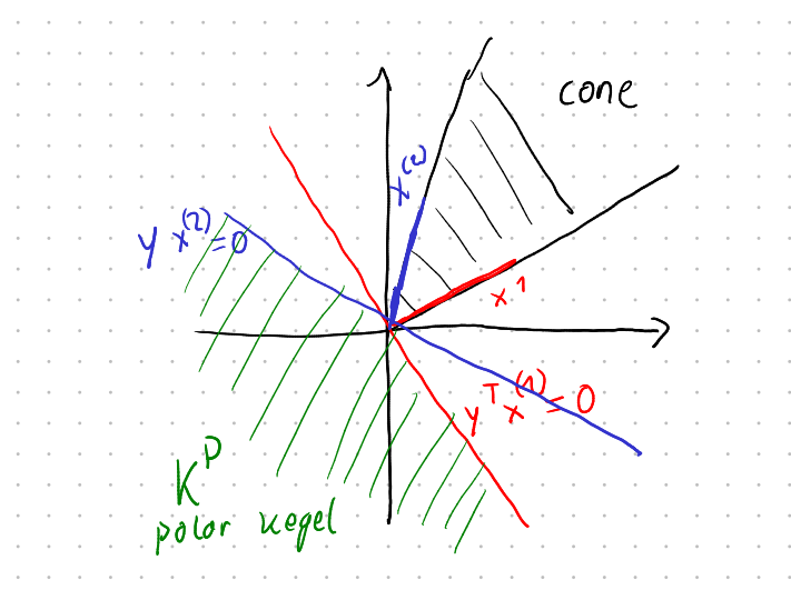
Solution b)
“\( \subseteq \)”
By the definition of the polar cone, we have:
\[ K^P = \{ y \in \mathbb{R}^n \mid y^\top x \leq 0 \text{ for all } x \in K \}. \]Since \( K = \text{cone} \{ x^{(1)}, \dots, x^{(m)} \} \), every element \( x \in K \) can be written as:
\[ x = \sum_{i=1}^{m} \lambda_i x^{(i)}, \quad \lambda_i \geq 0. \]Thus, if \( y \in K^P \), then for all such \( x \):
\[ y^\top x = y^\top \left( \sum_{i=1}^{m} \lambda_i x^{(i)} \right) = \sum_{i=1}^{m} \lambda_i (y^\top x^{(i)}) \leq 0. \]Since \( \lambda_i \geq 0 \), this implies \( y^\top x^{(i)} \leq 0 \) for all \( i \), proving:
\[ y \in \{ y \in \mathbb{R}^n \mid y^\top x^{(i)} \leq 0 \text{ for } i=1, \dots, m \}. \]“\( \supseteq \)”
Now, assume \( y \in \mathbb{R}^n \) satisfies:
\[ y^\top x^{(i)} \leq 0 \quad \text{for all } i=1, \dots, m. \]For any \( x \in K \), we write \( x \) as a conic combination:
\[ x = \sum_{i=1}^{m} \lambda_i x^{(i)}, \quad \lambda_i \geq 0. \]Applying the given inequality:
\[ y^\top x = y^\top \left( \sum_{i=1}^{m} \lambda_i x^{(i)} \right) = \sum_{i=1}^{m} \lambda_i (y^\top x^{(i)}). \]Since each \( \lambda_i \geq 0 \) and \( y^\top x^{(i)} \leq 0 \), it follows that:
\[ y^\top x \leq 0 \quad \forall x \in K. \]Thus, \( y \in K^P \), completing the proof.
Solution c)
Remember: Statement of Farkas’ Lemma
Farkas’ Lemma states that for a matrix \( A \), exactly one of the following holds for any \( x \in \mathbb{R}^n \):
- \( \exists \lambda \in \mathbb{R}^m, \lambda \geq 0 \) such that \( A \lambda = x \), or
- \( \exists y \in \mathbb{R}^n \) such that \( y^\top x \geq 0 \) and \( A^\top y \leq 0 \).
Let \( x \in K \):
\[ \begin{aligned} x \in K &\iff \exists \lambda_i \geq 0 \text{ such that } x = \sum_{i=1}^{m} \lambda_i x^{(i)} \\ &\iff \exists \lambda \geq 0 \text{ such that } A \lambda = x, \text{ where } A = \begin{bmatrix} x^{(1)} & x^{(2)} & \dots & x^{(m)} \end{bmatrix} \\ &\iff \forall y \in \mathbb{R}^n, \quad y^\top x \leq 0 \quad \text{(by Farkas' Lemma)} \\ &\iff \forall y \in K^P, \quad y^\top x \leq 0 \\ &\iff x \in (K^P)^P. \end{aligned} \]Thus, we conclude that \( (K^P)^P = K \).
Problem 44
Consider the extended version of the Rock-Paper-Scissors game that includes Lizard and Spock, with the following rules:
- Scissors beats Paper and Lizard.
- Rock beats Scissors and Lizard.
- Paper beats Rock and Spock.
- Spock beats Scissors and Rock.
- Lizard beats Paper and Spock.
(a) Construct the payoff matrix for this two-player matrix game, where a loss incurs a cost of 1.
(Reminder: A matrix entry represents the payoff for Player 1 and Player 2.)
Is the game fair?
(b) Show that the uniformly distributed strategies
\[ x^* = \begin{pmatrix} \frac{1}{5}, \frac{1}{5}, \frac{1}{5}, \frac{1}{5}, \frac{1}{5} \end{pmatrix}^T = y^* \]for Player 1 and Player 2 form a saddle point \((x^*, y^*)\).
(c) Are there optimal pure strategies for either Player 1 or Player 2?
Solution a)
The payoff matrix \( A \) is skew-symmetric, meaning:
\[ A^\top = -A. \]Since in a two-player zero-sum game, skew-symmetry implies that the expected payoff is always zero for optimal mixed strategies, the game is fair.
Solution b)
We need to show that \( (x^*, y^*) \) is a saddle point for the function:
\[ \phi(x, y) = y^\top A x, \quad \forall x, y \geq 0. \]That is, we must verify:
\[ \phi(x^*, y) \leq \phi(x^*, y^*) \leq \phi(x, y^*), \quad \forall x, y. \]Since the rows and columns of \( A \) sum to zero, we have:
\[ (y^*)^\top A = 0^\top, \quad Ax^* = 0. \]This means:
\[ \phi(x^*, y) = y^\top A x^* = 0, \quad \text{and} \quad \phi(x, y^*) = (y^*)^\top A x = 0. \]Thus, the saddle point equation holds, proving that \( (x^*, y^*) \) is indeed a saddle point.
Solution c)
We show that no pure strategy is optimal for either player.
Suppose Player 1 chooses a pure strategy indexed by \( p \) (\( p \in \{1, \dots, 5\} \)).
Then Player 2 can always find a pure counter-strategy \( q = q(p) \) such that:
The same reasoning holds in reverse: Player 2 choosing a pure strategy allows Player 1 to counter with a pure strategy ensuring a win.
Since both players can always counter any pure strategy of their opponent, no pure strategy is optimal.
Problem 45
Max and Mara want to camp in a Swedish national park. Mara prefers warmer locations, while Max prefers cooler ones, making it difficult to choose the right spot. The park contains \( m \in \mathbb{N} \) trails running east-west and \( n \in \mathbb{N} \) streams running north-south. They decide to camp at a ford, and as a compromise, Mara gets to choose the trail, while Max gets to choose the stream. Additionally, they have access to a park guide that provides the average annual temperatures (in °C) at each ford.
(a) Formulate this situation as a two-person matrix game. Mara aims to camp at a location with the highest possible average temperature, while Max tries to camp at a location with the *lowest possible average temperature
(b) Consider what would generally be interpreted as a fair outcome of this matrix game for a given “temperature matrix”.
(c) Consider the following example for \( m = n = 4 \), where the average annual temperatures at the fords are given in Table 1. Show that this results in a saddle-point game. Determine the corresponding pure optimal strategies and indicate where Mara and Max will camp if they follow these strategies.
\[ \begin{array}{c|cccc} \text{Trail} \backslash \text{Stream} & \text{Forellenbach} & \text{Froschbach} & \text{Moskitobach} & \text{Lachsbach} \\ \hline \text{Hasenweg} & -0.6 & -2.6 & -1.6 & -0.6 \\ \text{Fuchsweg} & -1.6 & 1.4 & -0.6 & 3.4 \\ \text{Elchweg} & -1.6 & 5.0 & -2.6 & -1.6 \\ \text{Hirschweg} & 1.4 & 3.4 & -0.6 & -0.6 \\ \end{array} \]Table 1: Average annual temperatures at the fords (in °C).
(d) Verify whether the matrix game from (c) is fair in the sense of part (b).
Solution a)
Let Max be Player 1 and Mara be Player 2, and let the payoff matrix \( A = (a_{ij}) \) represent the temperature at the intersection of the \(i\)-th trail and the \(j\)-th stream.
Max wants to minimize the maximum temperature across all streams, so the objective is:
\[ \text{minimize } \max_{y \geq 0} \, y^\top A x, \quad x \geq 0, \, e^\top x = 1 \]Mara, on the other hand, wants to maximize the minimum temperature across all trails, so the objective is:
\[ \text{maximize } \min_{x \geq 0} \, y^\top A x, \quad y \geq 0, \, e^\top y = 1 \]Solution b)
One could calculate the mean or median of the temperatures (from the matrix) as a fair outcome for the matrix game:
\[ (y^*)^\top A x^* = \bar{a} = \frac{1}{nm} \sum a_j \]Where \( \bar{a} \) represents the average temperature, and the sum \( \sum a_j \) is taken over all elements in the matrix \( A \).
Solution c)
Saddle-Point Game: A game with payoff matrix \( A \) is called a saddle-point game if the smallest maximum column entry and the largest minimum row entry coincide. For every saddle-point game, there are optimal pure strategies \( x^* = e_j \) and \( y^* = e_i \) (see Theorem 4.12).
Verification of the criterion:
\[ \min_j \max_i a_{ij} = \min_j \{1.4, 5, -0.6, 3.4\} = -0.6 \]\[ \max_i \min_j a_{ij} = \max_i \{-2.6, -1.6, -2.6, -0.6\} = -0.6 \]This shows that it is indeed a saddle-point game.
By Theorem 4.12, Player 1 should choose the column \( j_0 \) where the maximum is minimized, and similarly for Player 2:
\[ j_0 = \arg \min \max a_{ij} = 3 \]\[ i_0 = \arg \min \min a_{ij} = 4 \]Thus, the optimal strategies are \( x^* = e_3 \) and \( y^* = e_4 \). Therefore, Mara and Max should camp at the ford “Hirschung/Moskitobach.”
Solution d)
The resulting annual average temperature at the destination is \( -0.6^\circ \) Celsius. Since for this matrix, \( 0 = \bar{a} \neq 0.6 \), the matrix game is not fair in terms of the mean value.Problem 46
Let \( A \in \mathbb{R}^{m \times n} \), \( b \in \mathbb{R}^m \), and the polyhedron \( M = \{ x \in \mathbb{R}^n : Ax \leq b \} \) be non-empty. We are looking for the radius \( r \geq 0 \) and the center \( z \in \mathbb{R}^n \) such that the ball \( B_r(z) \) lies entirely within \( M \) and has the largest possible radius.
We want to show that this problem is equivalent to the following linear program:
\[ \text{Maximize } r \quad \text{subject to} \quad a_k^\top z + |a_k| r \leq b_k, \quad k = 1, \dots, m, \]where \( a_k^\top \) denotes the \( k \)-th row of the matrix \( A \).
Hint: Inner products can be estimated using the Cauchy-Schwarz inequality.
Solution
We consider the problem:
Maximize \( r \) subject to \( B_r(z) \subset M = \{x : Ax \leq b\} \).
We now rewrite the constraints as follows:
\[ B_r(z) \subset M \iff Ax \leq b \quad \forall x \in \mathbb{R}^n : |x - z| \leq r \]\[ \iff a_k^\top x \leq b_k \quad \forall x : |x - z| \leq r \]\[ \iff a_k^\top (y + z) \leq b_k \quad \forall y : |y| \leq r \quad (y := x - z, \, x := y + z) \]\[ \iff a_k^\top z + a_k^\top y \leq b_k \quad \forall y : |y| \leq r \]\[ \iff a_k^\top z + \max\{ a_k^\top y : |y| \leq r \} \leq b_k \]Since \( a_k^\top y \leq |a_k| |y| \) and equality holds for \( y = a_k \frac{|y|}{|a_k|} \), we obtain:
\[ B_r(z) \subset M \iff a_k^\top z + \max\{|a_k| |y| : |y| \leq r\} \leq b_k \]\[ \iff a_k^\top z + |a_k| r \leq b_k \]Problem 47
Let \( M \) be the triangle bounded by the positive \( x_1 \)- and \( x_2 \)-axes, as well as the line \( x_2 = -x_1 + 1 \). Determine the radius \( r^* \geq 0 \) and the center \( x^* \in \mathbb{R}^2 \) of the largest circle that fits entirely within \( M \) using the simplex method.
Solution
We use the result from Task 46. To calculate the triangle as a polyhedron, we have:
$$ M = \{ x \in \mathbb{R}^2 : A x \leq b \} $$with
$$ A = \begin{pmatrix} -1 & 0 \\ 0 & -1 \\ 1 & 1 \\ \end{pmatrix}, \quad b = \begin{pmatrix} 0 \\ 0 \\ 1 \end{pmatrix} $$The minimization problem is:
$$ \min -r \quad \begin{pmatrix} -1 & 0 & 1 \\ 0 & -1 & 1 \\ 1 & 1 & \sqrt{2} \end{pmatrix} (x_1 \ x_2 \ r)^T \leq \begin{pmatrix} 0 \\ 0 \\ 1 \end{pmatrix}, \quad x_1, x_2, r \geq 0 $$Now we can apply Phase 2 directly:
$$ \begin{bmatrix} 0 & 0 & -1 & 0 & 0 & 0 & | 0 \\ \hline -1 & 0 & 1 & 1 & 0 & 0 & | 0 \\ 0 & -1 & 1 & 0 & 1 & 0 & | 0 \\ 1 & 1 & \sqrt{2} & 0 & 0 & 1 & | 1 \end{bmatrix} $$We choose the pivot \( a_{13} = 1 \).
Now we can continue the Simplex algorithm.
The result is:
$$ r^* = \frac{1}{2 + \sqrt{2}}, \quad x^* = (r^*, r^*)^T $$Problems with Un-confirmed Solution
Problems in this section do not have an official solution, this means the provided solution could be wrong.
Problem 48
a) Show that the following sets are polyhedral
(i)
$$ M_1 := \{(x,y) \in \mathbb{R}^2 \ : \ max\{|x|, |y| \leq 1\}\} $$(ii)
$$ M_2 := \{(x,y) \in \mathbb{R}^2 \ : \ |x| + |y| \leq 1\} $$b) For \(\alpha, \beta \in \mathbb{R}\) is the following optimization problem given:
$$ (P) \quad \min \ \alpha x_1 + \beta x_2 \ \ \text{under} \ \ \begin{bmatrix} 1 & 1 \\ 2 & 1 \end{bmatrix} \begin{bmatrix} x_1 \\ x_2 \end{bmatrix} \begin{bmatrix} 2 \\ 1 \end{bmatrix}, \ \ x_1, x_2 \geq 0 $$(i) Formulate the dual problem (D) to (P).
(ii) Investigate with the strong dualitiy lemma, if the dual prolbem (D) is solvable.
Solution a)
(i) We can visuliaze \(M_1\) as follows
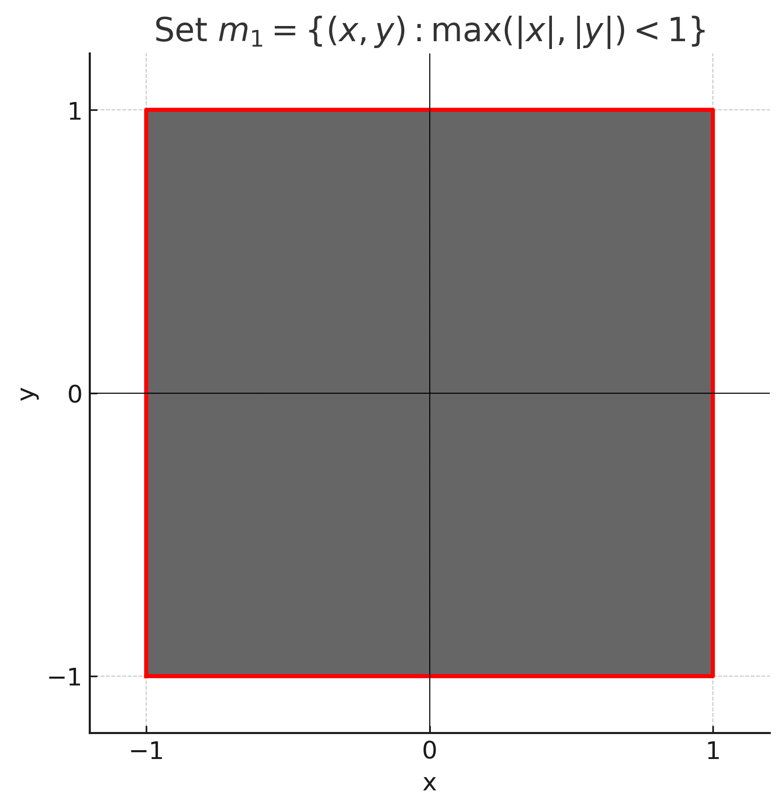
From the picture we can see that we can express the set with the following linear ineqliaities
$$ x \leq 1, \ x \geq -1, \ y \leq 1, \ y \geq -1 $$Hence we can write
$$ M_1 = \{(x,y) \in \mathbb{R}^2 \ : \ Az = b\} $$with
$$ A = \begin{bmatrix} 1 & 0 \\ -1 & 0 \\ 0 & 1 \\ 0 & -1 \end{bmatrix}, \ b = \begin{bmatrix} 1 \\ 1 \\ 1 \\ 1 \\ \end{bmatrix}, \ z = \begin{bmatrix} x \\ y \end{bmatrix} $$We have written \(M_1\) as an intersection of finitely many linear inequation, thus \(M_1\) is a polyhedral.
(ii) We can visuliaze \(M_1\) as follows
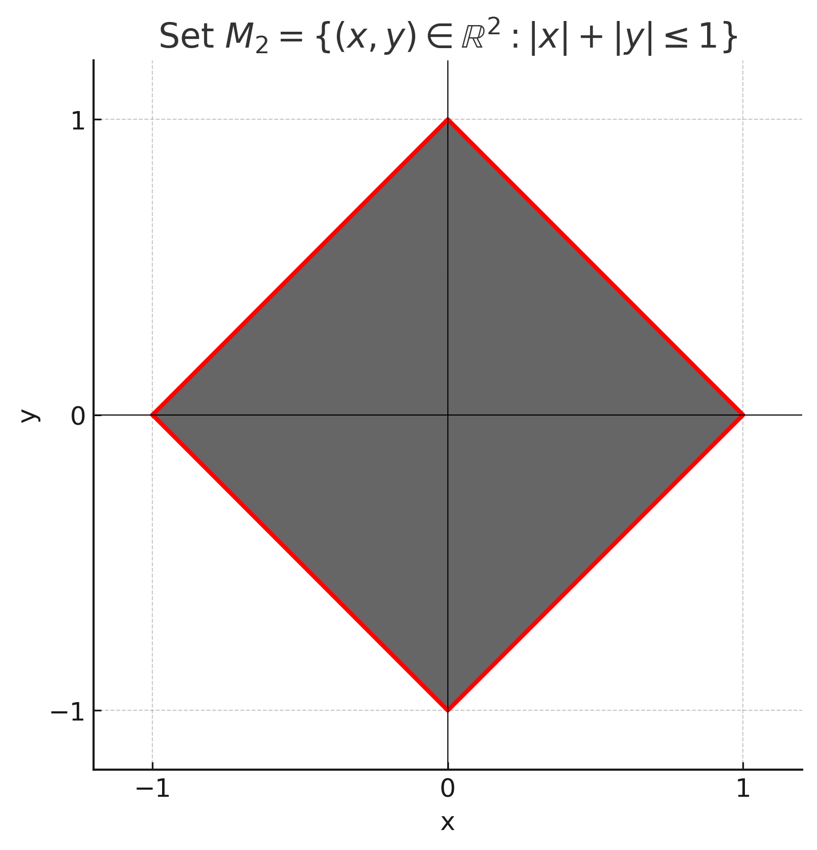
From the picture we can see that we can express the set with the following linear ineqliaities
$$ x + y \leq 1, \ x - y \leq 1, \ -x + y \leq 1, \ -x - y \leq 1 $$Hence we can write
$$ M_2 = \{(x,y) \in \mathbb{R}^2 \ : \ Az = b\} $$with
$$ A = \begin{bmatrix} 1 & 1 \\ 1 & -1 \\ -1 & 1 \\ -1 & -1 \end{bmatrix}, \ b = \begin{bmatrix} 1 \\ 1 \\ 1 \\ 1 \\ \end{bmatrix}, \ z = \begin{bmatrix} x \\ y \end{bmatrix} $$We have written \(M_2\) as an intersection of finitely many linear inequation, thus \(M_2\) is a polyhedral.
Solution b)
(i) The dual problem is given by
$$ (D) \quad \max 2x_1 + x_2 \ \ \text{under} \ \ \begin{bmatrix} 1 & 2 \\ 1 & 1 \end{bmatrix} \begin{bmatrix} y_1 \\ y_2 \end{bmatrix} \begin{bmatrix} \alpha \\ \beta \end{bmatrix} $$(ii) We use gaussian elimination on the restriction set of (P)
$$ \begin{bmatrix} 1 & 1 & | & 2 \\ 2 & 1 & | & 1 \end{bmatrix} \rightsquigarrow \begin{bmatrix} 1 & 1 & | & 2 \\ 1 & 0 & | & -1 \end{bmatrix} \implies x_1 = -1, \quad x_2 = 3 $$Thus we know that (P) is not feasible, because of the restriction \( x_1 \geq 0\).
We use gaussian elimination on the restriction set of (D)
$$ \begin{bmatrix} 1 & 2 & | & \alpha \\ 1 & 1 & | & \beta \end{bmatrix} \rightsquigarrow \begin{bmatrix} 0 & 1 & | & \alpha - \beta \\ 1 & 1 & | & \beta \end{bmatrix} \implies y_2 = \alpha - \beta, \quad y_1 = 2 \beta - \alpha $$Thus (D) is feasible.
Because (P) is not feasible and (D) is feasible we can use the lemma of strong duality, which gives us \(\sup(P) = +\infty\).
Problem 49
To earn some extra money, hobby baker Michi wants to sell his homemade cakes at the local weekly market. He offers a nut cake and a chocolate cake, both made from his secret cake mix, chocolate, and nuts. His recipes for each cake are as follows:
$$ \begin{array}{c|c|c} & \text{Nut Cake} & \text{Chocolate Cake} \\ \hline \text{Baking mix} & 0.8 & 0.8 \\ \text{Chocolate} & 0.1 & 0.2 \\ \text{Nuts} & 0.1 & - \\ \end{array} $$He can sell his nut cake for 6 Talers per piece and his chocolate cake for 8 Talers per piece. For the production of his cakes for the next market day, he has 100 kg of cake mix, 20 kg of chocolate, and 10 kg of nuts available. More ingredients that meet his quality standards were simply unavailable. Michi’s goal is to maximize his earnings for the next market day with the ingredients at hand.
a) Formulate the problem as an optimization problem using matrices.
b) Solve the problem using the simplex algorithmus. How many cakes of which type need to be sold and what amount to maximize profit?
c) Draw the restrictionset from (a) and mark all basis solutions from (b).
Solution a)
The optimizaton problem is as follows
$$ \min \ c^Tx \ \ \text{under} \ \ Ax \leq b, x \geq 0, x \in \mathbb{R}^2 $$where
$$ c = \begin{bmatrix} -6 \\ -8 \end{bmatrix}, \ A = \begin{bmatrix} 0.8 & 0.8 \\ 0.1 & 0.2 \\ 0.1 & 0 \end{bmatrix}, \ b = \begin{bmatrix} 100 \\ 20 \\ 10 \end{bmatrix} $$where \(x_1\) is the number of nut cakes and \(x_2\) is then umber of chocolate cakes.
Solution b)
We formulate the tabular of the simplex algorithm and introduce the slackvariables \(s_1, s_2, s_3 \geq 0\)
$$ T_0 : \ \ \begin{array}{ccccc|c} -6 & -8 & 0 & 0 & 0 & \gamma \\ \hline 0.8 & 0.8 & 1 & 0 & 0 & 100\\ 0.1 & 0.2 & 0 & 1 & 0 & 20 \\ \fbox{0.1} & 0 & 0 & 0 & 1 & 10 \end{array} $$We have the basis solution \((x_1, x_2, s_1, s_2, s_3) = (0, 0, 100, 20, 10)\), thus we can start with phase 2 of the ismplex algorithmn.
$$ T_1 : \ \ \begin{array}{ccccc|c} 0 & -8 & 0 & 0 & 0 & \gamma + 600 \\ \hline 0 & \fbox{0.8} & 1 & 0 & -8 & 20\\ 0 & 0.2 & 0 & 1 & -1 & 10 \\ 1 & 0 & 0 & 0 & 10 & 100 \end{array} $$We have the basis solution \((x_1, x_2, s_1, s_2, s_3) = (100, 0, 20, 10, 0)\).
$$ T_2 : \ \ \begin{array}{ccccc|c} 0 & 0 & 10 & 0 & -20 & \gamma + 800 \\ \hline 0 & 1 & 1.25 & 0 & -10 & 25 \\ 0 & 0 & -0.25 & 1 & \fbox{1} & 5 \\ 1 & 0 & 0 & 0 & 10 & 100 \end{array} $$We have the basis solution \((x_1, x_2, s_1, s_2, s_3) = (100, 25, 0, 5, 0)\).
$$ T_3 : \ \ \begin{array}{ccccc|c} 0 & 0 & 7.5 & 20 & 0 & \gamma + 900 \\ \hline 0 & 1 & -1.25 & 10 & 0 & 75 \\ 0 & 0 & -0.25 & 1 & 1 & 5 \\ 1 & 0 & 2.5 & 0 & 0 & 50 \end{array} $$Since the first row is now entirely postive we are finished with the simplex algorithm our final solution being \((x_1, x_2) = (50, 75)\) with a profit of \(f(x^*) = 900\) euro.
Solution c)
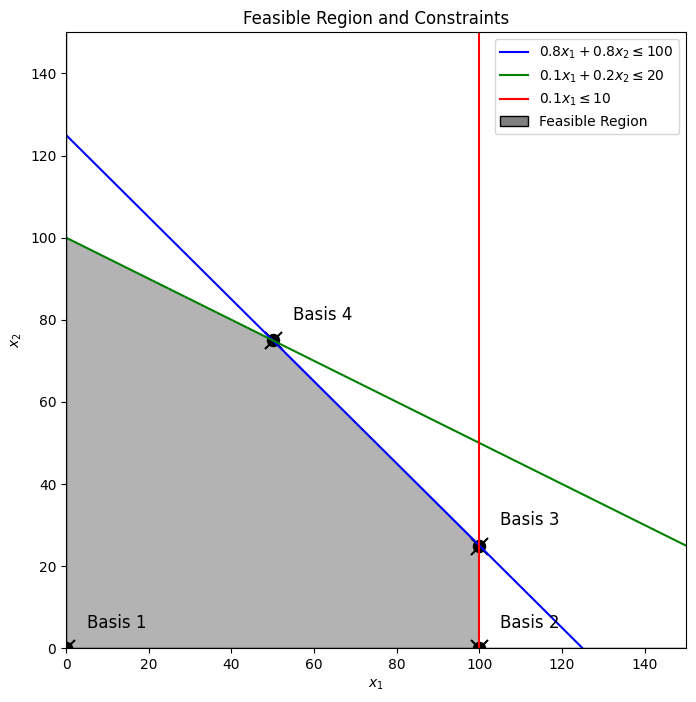
Python code for the diagram
<div class="highlight"><pre tabindex="0" class="chroma"><code class="language-python" data-lang="python"><span class="line"><span class="ln"> 1</span><span class="cl"><span class="kn">import</span> <span class="nn">numpy</span> <span class="k">as</span> <span class="nn">np</span>
2import matplotlib.pyplot as plt 3from matplotlib.lines import Line2D 4import matplotlib.patches as mpatches 5 6# Define the inequality constraints 7A = np.array([[0.8, 0.8], [0.1, 0.2], [0.1, 0]]) 8b = np.array([100, 20, 10]) 9 10# Define x1 and x2 ranges 11x1 = np.linspace(0, 150, 300) 12x2 = np.linspace(0, 150, 300) 13 14# Create a grid of (x1, x2) 15X1, X2 = np.meshgrid(x1, x2) 16 17# Calculate the values of the inequalities 18ineq1 = A[0, 0] X1 + A[0, 1] X2 - b[0] # 0.8x1 + 0.8x2 <= 100 19ineq2 = A[1, 0] X1 + A[1, 1] X2 - b[1] # 0.1x1 + 0.2x2 <= 20 20ineq3 = A[2, 0] X1 + A[2, 1] X2 - b[2] # 0.1x1 <= 10 21 22# Create the plot 23plt.figure(figsize=(8, 8)) 24 25# Plot the constraints using contour 26contour1 = plt.contour(X1, X2, ineq1, levels=[0], colors='blue') 27contour2 = plt.contour(X1, X2, ineq2, levels=[0], colors='green') 28contour3 = plt.contour(X1, X2, ineq3, levels=[0], colors='red') 29 30# Create a boolean mask for the feasible region (flip the inequalities to >= 0 for below the lines) 31feasible_region = (ineq1 <= 0) & (ineq2 <= 0) & (ineq3 <= 0) & (X1 >= 0) & (X2 >= 0) 32inverted_feasible_region = ~feasible_region 33 34# Plot the feasible region 35plt.imshow(inverted_feasible_region.astype(int), extent=[x1.min(), x1.max(), x2.min(), x2.max()], 36 origin='lower', cmap='gray', alpha=0.3, aspect='auto') 37 38# Setup labels and axes 39plt.xlim(0, 150) 40plt.ylim(0, 150) 41plt.axhline(0, color='black', linewidth=1) 42plt.axvline(0, color='black', linewidth=1) 43 44# Create the white rectangle for the feasible region 45feasible_patch = mpatches.Rectangle((0, 0), 1, 1, color='gray', ec='black', lw=1) 46 47# Define the legend handles 48legend_handles = [ 49 Line2D([0], [0], color='blue', label=r'$0.8x_1 + 0.8x_2 \leq 100$'), 50 Line2D([0], [0], color='green', label=r'$0.1x_1 + 0.2x_2 \leq 20$'), 51 Line2D([0], [0], color='red', label=r'$0.1x_1 \leq 10$'), 52 feasible_patch # Add the white rectangle to the legend handles 53] 54 55# Add the legend with the text for the feasible region 56plt.legend(handles=legend_handles, labels=[ 57 r'$0.8x_1 + 0.8x_2 \leq 100$', 58 r'$0.1x_1 + 0.2x_2 \leq 20$', 59 r'$0.1x_1 \leq 10$', 60 'Feasible Region' # The text for the white rectangle 61]) 62 63# Plot the labeled points 64points = np.array([[0, 0], [100, 0], [100, 25], [50, 75]]) 65labels = ['Basis 1', 'Basis 2', 'Basis 3', 'Basis 4'] 66 67# Plot the filled circles first 68plt.scatter(points[:, 0], points[:, 1], color='black', marker='o', s=75, edgecolor='black') # Circle 69 70# Overlay the 'x' markers 71plt.scatter(points[:, 0], points[:, 1], color='black', marker='x', s=150) # 'x' on top 72for i, (x, y) in enumerate(points): 73 plt.text(x + 5, y + 5, labels[i], fontsize=12, color='black') # Label the points with a small offset 74 75plt.title('Feasible Region and Constraints') 76plt.xlabel(r'$x_1$') 77plt.ylabel(r'$x_2$') 78 79plt.show()

 reply via email