Optimization Theory

January 23, 2025 | 21,807 words | 103min read

0. Motivation

I am currently studying computer science in Germany. In addition to the mandatory and elective courses that each student must complete, one is also required to choose a supplementary subject. This subject is unrelated to one’s major and can be anything from electrical engineering, mathematics, philosophy, psychology, or any other field. It can be compared to a minor in the American university system, with the key difference being that only a minimum of 10 ECTS credits are required, compared to the 30 ECTS typically required in the U.S.

When it came time to choose my supplementary subject, I chose mathematics with the idea of strengthening my foundation and gaining a deeper understanding of my passion for cognitive systems. The first course I took was Introduction to Algebra and Number Theory, which, despite the enormous effort and time I invested, I failed miserably. Consequently, I decided to select easier courses for my next attempts—one of which was Markov Chains, which I am embarrassed to say I barely passed, and Optimization Theory, which I unfortunately failed as well.

I have to retake Optimization Theory this semester, so I thought it would be a good opportunity to write an article about its content.

For a broader motivation as to why this subject might be interesting, look no further than today’s biggest trend: AI. But what exactly is AI? If you ask a dozen people, you might get two dozen answers. But broadly speaking, AI refers to creating systems that exhibit intelligent behavior. At the forefront of this field are deep learning models, which process vast amounts of data to generate models that can accurately predict outcomes within specific capabilities—for example, models such as Llama, DeepSeek, or Flux.

All of these AI models can, in a very strict sense, be considered optimization-theoretical problems. Given the vast amount of data, the challenge is to design a model that produces outputs aligned with the input data. Although I will not specifically cover the methodology of gradient descent, which is commonly used in such models, gaining a solid foundation in optimization theory will provide deeper insights into topics like gradient descent in the future.

1. Introduction

1.1 Example Problems

Example 1: Machine Occupancy Problem

In a workshop, we have two types of workpieces that can be produced on three types of machines. The running time for machines \(M_1, M_2, M_3\) for the workpieces \(E_1, E_2\) is known. What is the maximum number of workpieces that we can produce?

Machines	\(E_1\) h/piece	\(E_2\) h/piece	Running Time
\(M_1\)	10	10	8000
\(M_2\)	10	30	18000
\(M_3\)	20	10	14000

We want to create a mathematical model that describes the different constraints. For example, for workpieces \(E_1\) and \(E_2\), we derive the following constraint for machine \(M_2\):

$$ 10 E_1 + 30 E_2 \leq 18000 $$

We also need to ensure that \(E_1, E_2 \geq 0 \) since we cannot have a negative number of workpieces. With that, our complete model is:

$$ \begin{align} 10 E_1 + 10 E_2 &\leq 8000 \\ 10 E_1 + 30 E_2 &\leq 18000 \\ 20 E_1 + 10 E_2 &\leq 14000 \\ E_1, E_2 &\geq 0 \end{align} $$

We can summarize a possible solution for \(E_1, E_2\) using a vector:

$$ x = \begin{pmatrix} E_1 \\ E_2 \end{pmatrix} $$

Some possible solutions for the problem above include:

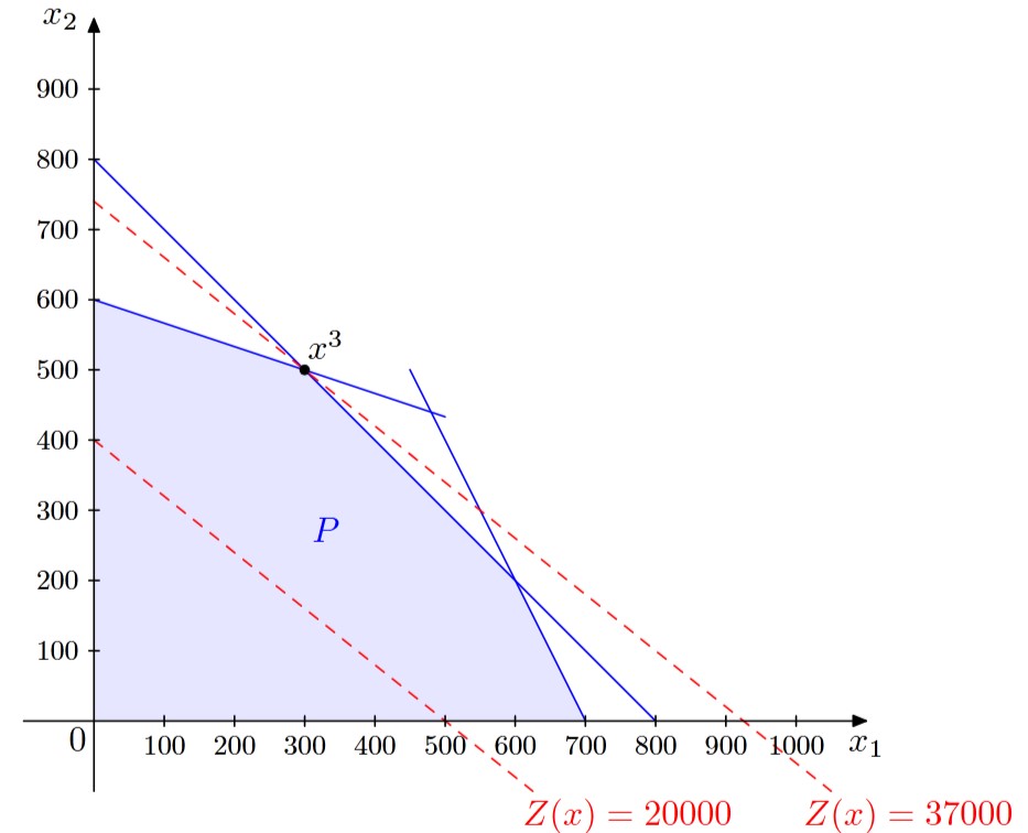
$$ x^1 = \begin{pmatrix} 700 \\ 0 \end{pmatrix}, \quad x^2 = \begin{pmatrix} 0 \\ 600 \end{pmatrix}, \quad x^3 = \begin{pmatrix} 300 \\ 500 \end{pmatrix} $$

These are valid solutions because we can substitute them into our model and verify that all inequalities are satisfied.

We want to refine our model further. Let’s say the manufacturing times for the workpieces are different, with \(E_1\) taking 40 hours and \(E_2\) taking 50 hours. Then, we can ask the question: what is the best possible solution under all given constraints? Formally, we can write this as:

$$ \begin{aligned} \max \quad & 40 E_1 + 50 E_2 \\ \text{subject to} \quad & 10 E_1 + 10 E_2 \leq 8000 \\ & 10 E_1 + 30 E_2 \leq 18000 \\ & 20 E_1 + 10 E_2 \leq 14000 \\ & E_1, E_2 \geq 0 \end{aligned} $$

This means that among all possible solutions \(x\), we want to find the one that maximizes \( Z(x) := 40 E_1 + 50 E_2 \). We call \(Z(x)\) the objective function, and the inequalities represent the set of constraints.

We can now substitute our possible solutions into \(Z(x)\). For example:

$$ Z(x^1) = 40 \times 700 + 50 \times 0 = 28000 $$

This means that if we produce 700 workpieces of \(E_1\) and 0 workpieces of \(E_2\), the total running time required for our machines would be 28,000 hours. By inserting our other possible solutions into \(Z(x)\), we find that \(x^3\) is the best solution from the given set. It is, in fact, the most optimal solution, which we will confirm later.

Example 2: Paint Production

A company produces four different types of paint: \(P_1, P_2, P_3,\) and \(P_4\). The respective profits per kilogram are 1.50€, 1€, 2€, and 1.40€. The company can produce a maximum of 1300 kg of paints \(L_1\) and \(L_2\), and a total of 2000 kg of \(L_1, L_3,\) and \(L_4\). Additionally, they must produce at least 800 kg of \(L_3\), and they know that they will never need more than 500 kg of \(L_4\).

The goal is to determine the optimal production quantities for each type of paint to achieve the highest possible profit.

The objective function to maximize profit is:

$$ z = 1.5 l_1 + l_2 + 2 l_3 + 1.4 l_4 $$

Subject to the following constraints:

$$ \begin{aligned} l_1 + l_2 &\leq 1300 \\ l_1 + l_3 + l_4 &\leq 2000 \\ l_3 &\geq 800 \\ l_4 &\leq 500 \end{aligned} $$

Additionally, the production amounts cannot be negative:

$$ l_i \geq 0, \quad (i = 1,2,3,4) $$

Example 3: Stigler’s Nutrition Model

In 1945, Stigler focused on the problem of minimizing the cost of an average man’s daily diet while meeting the required nutritional needs. For his study, he analyzed 77 different foods, examining their nutritional content and costs. The table below presents a selection of the foods and their corresponding nutrient values.

Food Item	Calories (1000)	Protein (g)	Calcium (g)	Iron (mg)	Vitamin-A (1000 iu)	Vitamin-B1 (mg)	Vitamin-B2 (mg)	Niacin (mg)	Vitamin-C (mg)
Wheat	44.7	1411	2.0	365	55.4	33.3	441
Cornmeal	36	897	1.7	99	30.9	17.4	7.9	106
Canned Milk	8.4	422	15.1	9	26	3	23.5	11	60
Margarine	20.6	17	0.6	6	55.8	0.2
Cheese	7.4	448	16.4	19	28.1	0.8	10.3	4
Peanut-B	15.7	661	1	48	9.6	8.1	471
Lard	41.7			0.2		0.5	5
Liver	2.2	333	0.2	139	169.2	6.4	50.8	316	525
Pork Roast	4.4	249	0.3	37	18.2	3.6	79
Salmon	5.8	705	6.8	45	3.5	1	4.9	209
Green Beans	2.4	138	3.7	80	69	4.3	5.8	37	862
Cabbage	2.6	125	4.0	36	7.2	9.0	4.5	26	5369
Onions	5.8	166	3.8	59	16.6	4.7	5.9	21	1184
Potatoes	14.3	336	1.8	118	6.7	29.4	7.1	198	2522
Spinach	1.1	106		138	918.4	5.7	13.8	33	2755
Sweet Potatoes	9.6	138	2.7	54	290.7	8.4	5.4	83	1912
Peaches	8.5	87	1.7	173	86.8	1.2	4.3	55	57
Prunes	12.8	99	2.5	154	85.7	3.9	4.3	65	257
Lima Beans	17.4	1055	3.7	459	5.1	26.9	38.2	93
Navy Beans	26.9	1691	11.4	792		38.4	24.6	217
Requirements	3000	70	0.8	12	5000	1.8	2.7	18	75

Source: diet.gms : Stigler's Nutrition Model

The nutritional requirements in the last row correspond to a man weighing 70 kg with an average level of activity. The table is normalized so that each unit of measurement costs exactly $1. Thus, the problem can be solved by minimizing the total cost of the selected food items.

Stigler found that an optimal diet cost only $39.90 per year, which amounts to less than 11 cents per day. Remarkably, the optimal solution required only 10 different types of food.

1.2 From the Model to the Solution

All the problems we have seen so far have one thing in common: we have a linear function that we want to minimize, subject to a set of linear constraints. Such problems are called linear optimization problems or linear programs (short LP).

Every optimization problem consists of five distinct phases:

1. Find an appropriate mathematical optimization model for the task at hand.
2. Simplify the mathematical model as much as possible.
3. Collect data that accurately describes the concrete task.
4. Apply a suitable method to find a solution.
5. Interpret the solution.

In practice, this is an iterative process.

2. Geometry of Linear Programs

The set of solutions for an optimization problem has important characteristics, which can significantly simplify the search for the optimal solution.

2.1 The Canonical Form of Linear Programming

We can represent a solution to an optimization problem as a vector \(x \in \mathbb{R}^n\) with \(n\) components. The objective function \(z(x)\) can be described using the coefficients \(c_0, c_1, c_2, ..., c_n \in \mathbb{R}\):

$$ z(x) = c_0 + c_1 x_1 + c_2 x_2 + \dots + c_n x_n $$

We can represent the column vector as a row vector \(c\) through transposition:

$$ c^T := (c_1, c_2, ..., c_n) $$

Using matrix multiplication, we can then calculate the value of \(z(x)\) as:

$$ z(x) = c_0 + c^T x $$

A system of inequalities, like our constraint set, can be written as:

$$ \begin{aligned} a_{11} x_1 + a_{12} x_2 + \dots + a_{1n} x_n &\leq b_1 \\ a_{21} x_1 + a_{22} x_2 + \dots + a_{2n} x_n &\leq b_2 \\ \vdots \\ a_{m1} x_1 + a_{m2} x_2 + \dots + a_{mn} x_n &\leq b_m \\ x_1, x_2, \dots, x_n &\geq 0 \end{aligned} $$

This can be described by a matrix \(A\) for the coefficients of the inequalities and a column vector \(b\):

$$ A = \begin{pmatrix} a_{11} & a_{12} & \cdots & a_{1n} \\ a_{21} & a_{22} & \cdots & a_{2n} \\ \vdots & \vdots & \ddots & \vdots \\ a_{m1} & a_{m2} & \cdots & a_{mn} \\ \end{pmatrix}, \quad b = \begin{pmatrix} b_1 \\ b_2 \\ \vdots \\ b_m \end{pmatrix}. $$

In summary, we can describe the constraint set of our linear program as:

$$ Ax \leq b, \quad x \geq 0 $$

This is also called the valid/feasible solution set. Furthermore, we can describe our optimization problem as:

$$ \max\{ c_0 + c^T x \ | \ Ax \leq b, x \geq 0 \} $$

We can omit the constant \(c_0\) since it does not affect the result of the solution. This formulation is called the canonical form. The set

$$ M = \{ x \in \mathbb{R}^n \ | \ Ax \leq b, x \geq 0 \} $$

is called the set of possible valid/feasible solutions, or simply the valid/feasible set.

Lemma Existence of Solution

Let \(K \neq \emptyset\) be compact and \(f : K \to \mathbb{R}\) continuous. Then has the the following optimization problem a global solution

$$ (P) \quad \min f(x) \ \ \text{on} \ \ x \in K $$

A set is compact, if it is closed (i.e. it contains all of its limits points) and bounded (i.e. it has a boundary).

A function is continuous, if the function is a single unbroken curve. A function is continious if it is a composition of continious functions.

2.2 Transformation into Canonical Form

Not all optimization problems are initially in canonical form. Some problems may look different, and we first need to transform them into the canonical form.

1. Minimizing \(c^T x\) is equivalent to maximizing \((-c)^T x\).
2. An inequality \(a^T x \geq b\) can be replaced by \((-a)^T x \leq -b\).
3. An equality \(a^T x = b\) can be replaced by two inequalities: \(a^T x \geq b\) and \(a^T x \leq b\).
4. If we have a variable \(x_j\) that is not necessarily positive, we can replace it with a pair of positive variables: \(x_j = x_j^+ - x_j^-\), where both \(x_j^+\) and \(x_j^-\) are non-negative.

By applying these transformations, any linear programming problem can be converted into canonical form.

2.3 Linear Function, Lines, Half-Spaces, and Polyhedral Spaces

The linear objective function and the set of valid/feasible solutions in an optimization problem have many important properties. This section examines a few of these properties.

Two points \(u, v\) define a line:

$$ L := \{u + \lambda (u - v) \ | \ \lambda \in \mathbb{R} \} $$

The linear objective function \(z(x) := z_0 + c^T x\) can be described as \(z(x) = z_0 + c^T(u + \lambda (x))(u - v)\).

We call a set \(K\) a cone if for every \(x \in K\) and \(\lambda \geq 0\), the following holds: \(\lambda x \in K\). A conic hull, denoted by \(cone(S)\), for a set \(S\) is the set of all conic combinations of the points in \(S\), i.e.,

$$ cone(S) = \left\{\sum_i \alpha_i x_i \ \middle| \ \alpha_i \geq 0, x_i \in S \right\} $$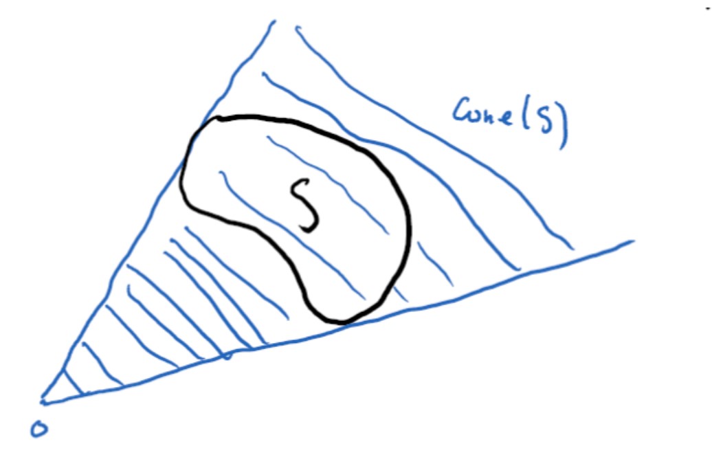

The sets of solutions:

$$ H_1 := \{x \ | \ a^T x \leq b \}, \quad H_2 := \{x \ | \ a^T x < b \} $$

\(H_1\) is called a closed half-space, and \(H_2\) is called an open half-space. Both are limited by the hyperplane:

$$ H_3 = \{x \ | \ a^T x = b \} $$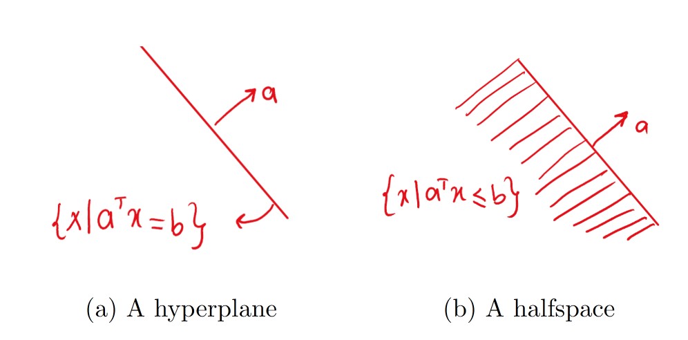

The intersection of a finite number of half-spaces is called a polyhedral space.

Importantly, the valid solutions of a linear program form a polyhedral space.

2.4 Geometrical Depiction of Two Variables

Let’s consider the following optimization problem in two dimensions:

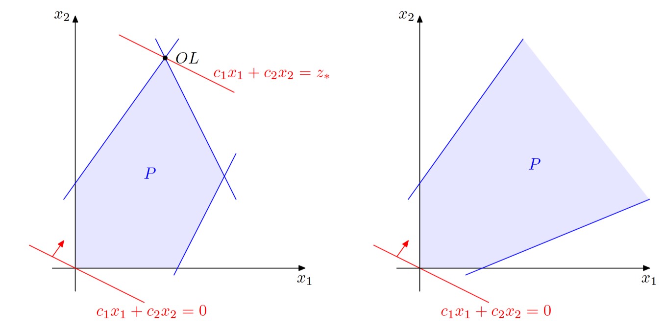
$$ \begin{aligned} \max \quad & c_1 x_1 + c_2 x_2 \\ \text{subject to} \quad & a_{i1} x_1 + a_{i2} x_2 \leq b_i, \quad (1 \leq i \leq m) \\ & x_1, x_2 \geq 0 \end{aligned} $$

The set of solutions that satisfy the inequalities forms a polyhedral space \(P\). A given inequality \(\{x \ | \ a_1 x_1 + a_2 x_2 \leq b\}\) represents a closed half-space, which is referred to as a half-plane in two dimensions. The intersection of these half-planes forms the set \(P\).

The intersection of half-spaces can be either empty or unrestricted, as shown below:

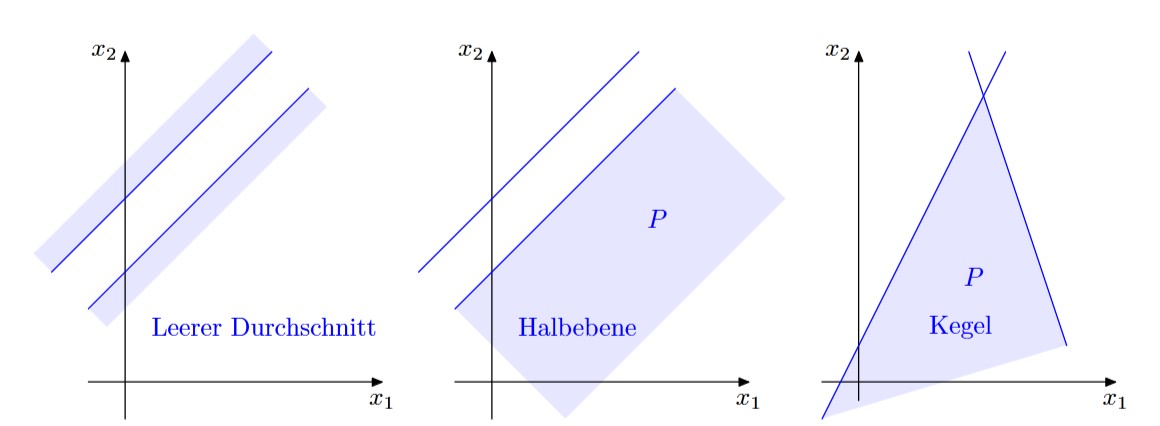
Furthermore, \(P\) can either be empty, unrestricted, or restricted, as seen below:

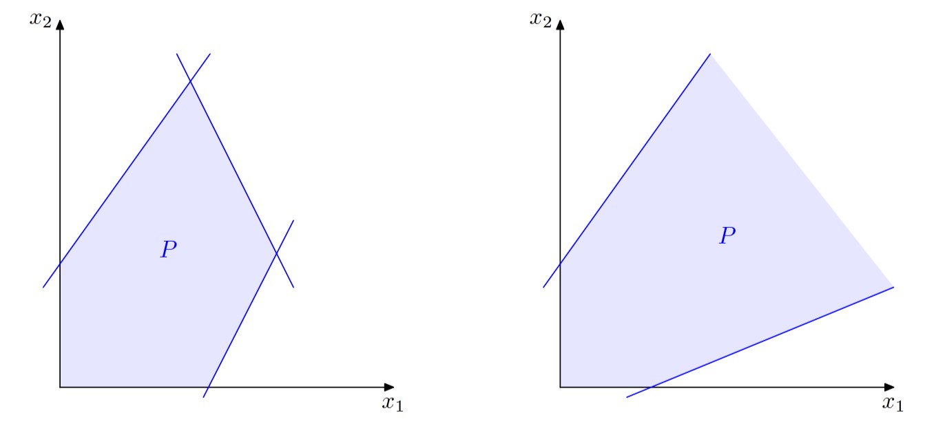
The objective function can be thought of as a shear between lines \(\{ x \ | \ c_1 x_1 + c_2 x_2 = z\}\), where \(z \in \mathbb{R}\). The goal of an optimization problem is to find where \(z\) achieves its maximum value, while still being within the region \(P\); in other words, the intersection between the objective function and the feasible region should not be empty.

Thus, we can solve a linear program graphically in two dimensions. However, this method of solution finding does not work in higher dimensions. Therefore, we need a method that works in higher dimensions as well.

2.5 Weyl and Farkas Lemma

The following are famous lemmas in the theory of polyhedra.

Lemma: Weyl
Every finite convex cone is polyhedral, and can be written in the form \( \{x \in \mathbb{R}^n : Ax \leq 0\} \). Therefore, finite convex cones are closed.

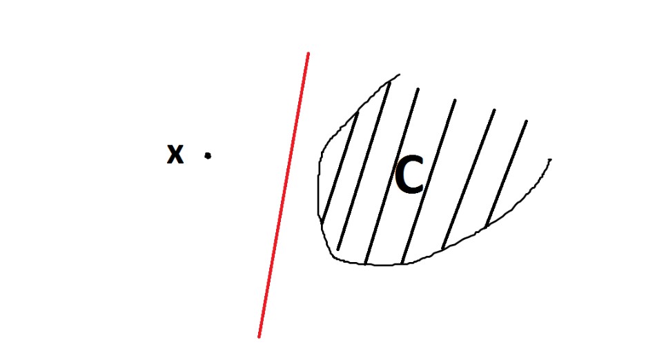
Lemma: Separation
Let \(C \subset \mathbb{R}^n\) be a convex, closed set, with \(C \neq \emptyset \), and let \(x \notin C\). Then, there exists a hyperplane that separates \(x\) and \(C\). In other words, there exists a vector \(a \in \mathbb{R}^n\), \(a \neq 0\), and a scalar \(\gamma \in \mathbb{R}\) such that:

$$ a^T z \leq \gamma \leq a^T x $$

If \(C\) is a convex cone, then \(\gamma = 0\) can be chosen.

This lemma means that if we have a closed set, we can always find a hyperplane that separates the convex set from the points outside the set.

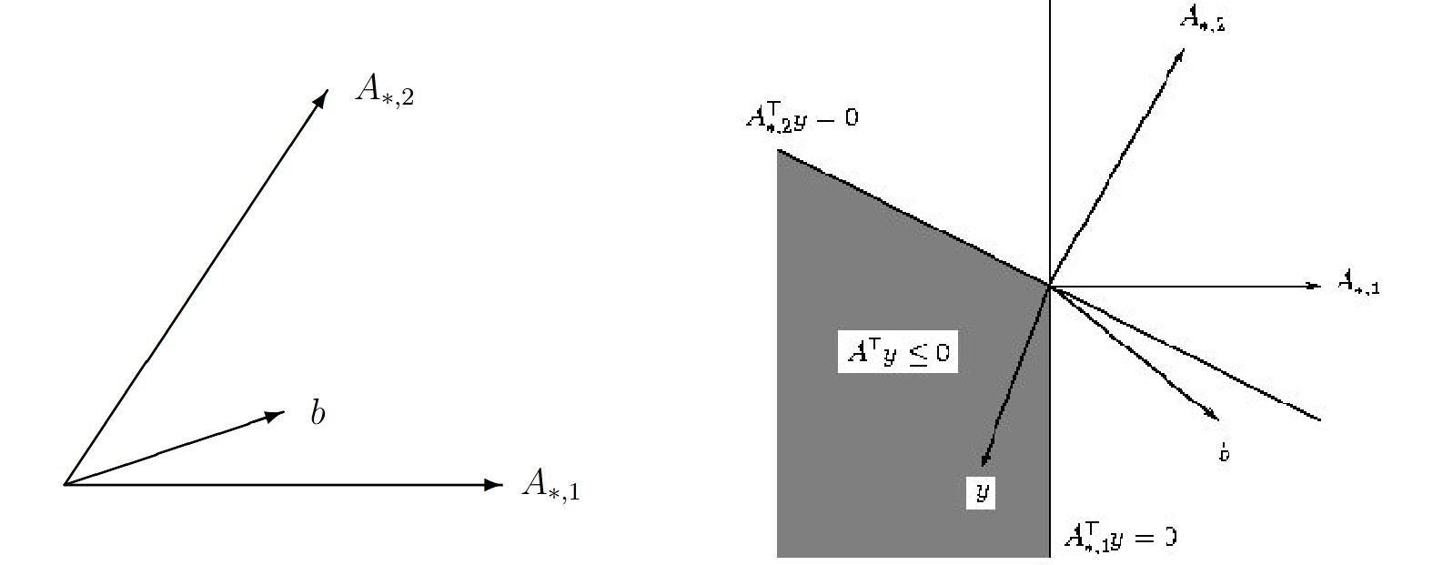
Lemma: Farkas
Let \(A \in \mathbb{R}^{m \times n}, b \in \mathbb{R}^m\). Then, one of the following statements is true, and the other false:
(i) The equation \(Ax = b, \ x \geq 0\) has a solution \(x \in \mathbb{R}^n\).
(ii) The system \(A^Ty \leq 0, \ b^Ty > 0\) has a solution \(y \in \mathbb{R}^m\).

2.6 The Main Theorem of Linear Programming

Now, let’s think about what points are optimal in a linear function on a non-empty polyhedral space.

The first claim is that every line-free polyhedron is the convex hull of its corners and extremal directions.

Definition
\(x \in M\) is called a corner or extremal point of \(M\) if \(x\) cannot be represented as a convex combination of two different points from \(M\). In other words:

$$ y, z \in M, \quad \lambda \in (0,1), \quad x = \lambda y + (1- \lambda) z \implies y = z $$

Definition
A vector \(u \in \mathbb{R}^n\) is called an extremal direction of \(M\) if the set \(\{ x + t u : t \geq 0 \} \subset M\) holds. Furthermore, \(u\) cannot be represented as a convex combination of two independent directions. In other words:

$$ \begin{aligned} v, w \text{ directions}, \quad \lambda \in (0,1), \quad u = \lambda v + (1-\lambda) w \\ \implies v, w \text{ are linearly independent}. \end{aligned} $$

Next, we state a result that characterizes the corners and extremal directions of a polyhedron.

Lemma
Let \( M = \{Ax \leq b\} \), and define the set of active indices \(I(x) := \{ i \in \{1, \dots, m\} : (Ax)_i = b_i \}\) for \(x \in M\). Then the following hold:

(a) \(x \in M\) is a corner of \(M\) if and only if \( \text{span}\{A_i^T : i \in I(x)\} = \mathbb{R}^n \), where \(A_i^T\) is the \(i\)-th row of \(A\).

(b) \(M\) has a finite number of corners.

(c) \(u \in \mathbb{R}^n\) is an extremal direction of \(M\) if and only if \(Au \leq 0\) and there are no other linearly independent directions \(v \in \mathbb{R}^n\) such that \(u = \lambda v + (1-\lambda) w\).

This lemma gives us important information: the set of valid solutions to our optimization problem has a finite number of corners, and we can find these corners by checking whether the active indices of a point form a span that equals \(\mathbb{R}^n\).

Lemma
Let \( M = \{Ax \leq b\} \) be a polyhedron and \(S \subset M\) be a side of \(M\). Then:

(a) Every corner of \(S\) is also a corner of \(M\).

(b) Every corner of \(S\) is an extremal direction of \(M\).

Finally, we can formulate the main theorem of linear programming:

Main Theorem
Let \(M \subset \mathbb{R}^n\) be a line-free polyhedron. Then:

$$ M = \text{conv} \{ \text{extr}(M) \cup \text{extr directions}(M) \} $$

In other words, \(M\) is the convex hull of its corners and extremal directions.

From this, we deduce:

Corollary
Let \(M \subset \mathbb{R}^n\) be a line-free polyhedron. Then \(M\) has exactly as many corners as it has no lines.

2.7 Set of Problems and Solutions

2.7.1 Transforming the Problem into Canonical Form

Task: Given the optimization problem:

\[ \text{maximize} \quad 5x_1 + x_2 - 2x_3 \]

under the constraints:

\[ x_1 \geq 0, \quad x_2 \leq 0, \quad x_3 \geq 0, \quad x_1 + 2x_2 + 3x_3 = 6, \]

bring it into the canonical form:

\[ (P) \quad \min \ c^T x, \quad M = \{ A x \leq b \} \]

Solution

We start by rewriting the constraints:

\[ \begin{aligned} -x_1 &\leq 0 \\ x_2 &\leq 0 \\ -x_3 &\leq 0 \\ x_1 + 2x_2 + 3x_3 &\leq 6 \\ -x_1 - 2x_2 - 3x_3 &\leq -6 \end{aligned} \]

Next, we rewrite the objective function \( 5x_1 + x_2 - 2x_3 \) as a minimization problem. To convert a maximization problem into a minimization problem, we negate the coefficients of the objective function, giving us:

\[ c = (-5, -1, 2)^T \]

Now, we have the canonical form:

\[ \min \ (-5, -1, 2)^T \begin{pmatrix} x_1 \\ x_2 \\ x_3 \end{pmatrix} \]

under the constraints:

\[ \begin{pmatrix} 1 & 0 & 0 \\ 0 & 1 & 0 \\ 0 & 0 & -1 \\ 1 & 2 & 3 \\ -1 & -2 & -3 \end{pmatrix} \begin{pmatrix} x_1 \\ x_2 \\ x_3 \end{pmatrix} \leq \begin{pmatrix} 0 \\ 0 \\ 0 \\ 6 \\ -6 \end{pmatrix} \]

2.7.2 Transforming the Problem into Canonical Form

Task: Given the optimization problem:

\[ \text{minimize} \quad x_1 - 2x_2 + 3x_3 \]

under the constraints:

\[ x_1 - x_2 \leq 1, \quad 3x_2 - 4x_3 \leq 5, \]

bring it into the canonical form:

\[ (P) \quad \min \ c^T x, \quad M = \{ A y = b, \, y \geq 0 \} \]

Solution

To ensure that all variables are non-negative, we introduce new variables \( u_i \) and \( v_i \) for each of \( x_1, x_2, x_3 \), such that:

\[ x_1 = u_1 - v_1, \quad x_2 = u_2 - v_2, \quad x_3 = u_3 - v_3, \]

where \( u_i, v_i \geq 0 \). With this, all variables are now non-negative. We can then rewrite the constraints as:

\[ \begin{aligned} u_1 - v_1 - u_2 - v_2 &\leq 1, \\ 3(u_2 - v_2) - 4(u_3 - v_3) &\leq 5. \end{aligned} \]

Next, we introduce slack variables \( y_1, y_2 \geq 0 \) to turn the inequalities into equalities:

\[ \begin{aligned} u_1 - v_1 - u_2 - v_2 + y_1 &= 1, \\ 3(u_2 - v_2) - 4(u_3 - v_3) + y_2 &= 5. \end{aligned} \]

The objective function needs to be transformed as well. The new objective function becomes:

\[ c = (1, -1, -2, 2, 3, -3, 0, 0). \]

Finally, we express the problem in canonical form as:

\[ \begin{pmatrix} 1 & -1 & -1 & -1 & 0 & 0 & 1 & 0 \\ 0 & 0 & 3 & -3 & -4 & 4 & 0 & 1 \end{pmatrix} y = \begin{pmatrix} 1 \\ 5 \end{pmatrix} \]

2.7.3 Feasibility

Task: Construct a linear problem with the form:

\[ (P) \quad \text{Minimize} \ \ c^T \ \text{subject to} \ Ax \leq b \]

So that:

• (a) (P) has no feasible points
• (b) (P) has exactly one feasible point
• (c) (P) is feasible, but \(\inf(P) = - \infty\)

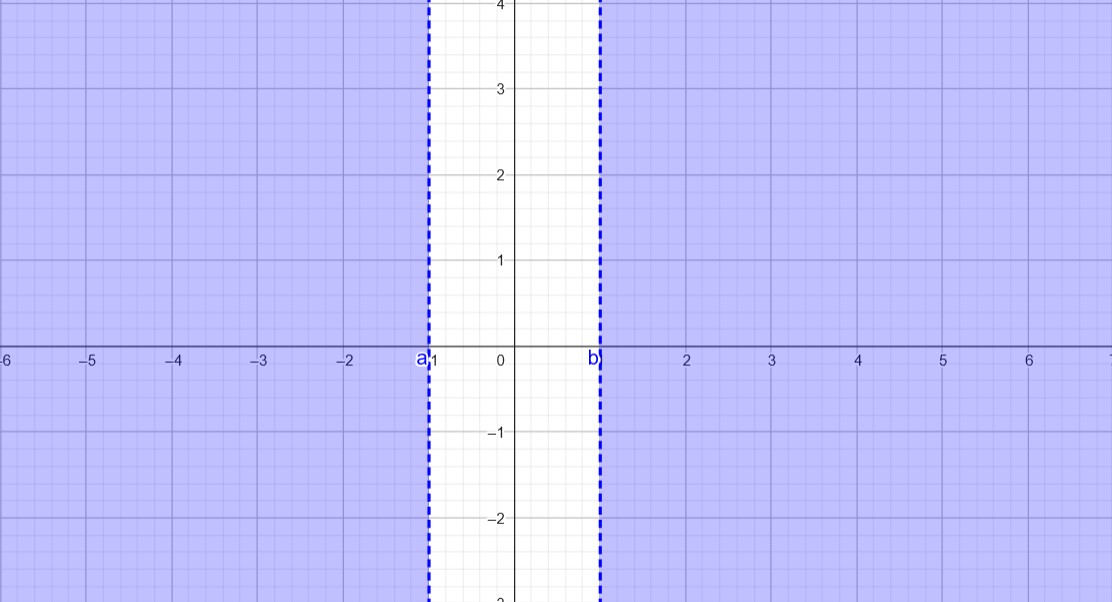
Solution (a)

In order to have no feasible points, the constraint set needs to be empty. This can be achieved by having one inequality that allows all points before \(-1\) and another inequality that allows all points after \(1\), which results in an empty intersection.

Constraints:

\[ \begin{aligned} x_1 &\leq -1 \\ x_1 &\geq 1 \end{aligned} \]

This can be represented in matrix form as:

\[ \begin{pmatrix} 1 & 0 \\ -1 & 0 \\ \end{pmatrix} x \ = \ \begin{pmatrix} -1 \\ 1 \end{pmatrix} \]

The intersection of these inequalities is empty, as shown in the illustration below:

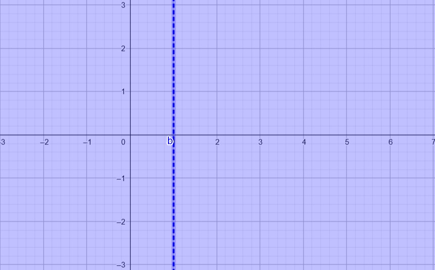
Solution (b)

To have exactly one feasible point, we need three inequalities. With two inequalities, we can have the x-axis in the feasible set, and by adding a third inequality, we can target a specific point, such as \((0,0)\).

Constraints:

\[ \begin{aligned} x_2 &\leq 0 \\ x_2 &\geq 0 \\ x_1 + x_2 &\geq 0 \end{aligned} \]

This can be represented in matrix form as:

\[ \begin{pmatrix} 0 & 1 \\ 0 & -1 \\ -1 & -1 \end{pmatrix} x \ = \ \begin{pmatrix} 0 \\ 0 \\ 0 \end{pmatrix} \]

The feasible set in this case consists of exactly one point, as shown in the illustration below:

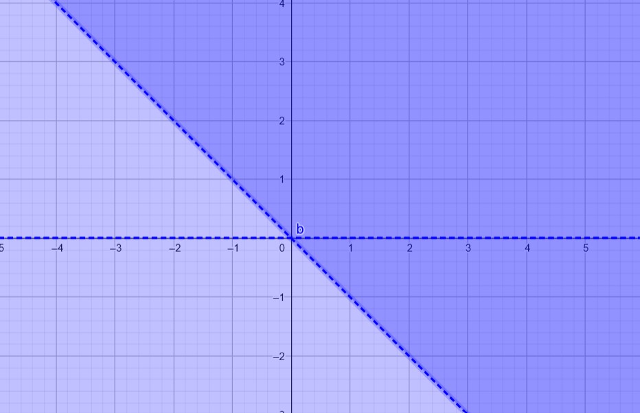
Solution (c)

To make the objective function unbounded, the feasibility set needs to be a line, and the objective function should optimize only one of the variables (e.g., \(x_2\)).

Constraints:

\[ \begin{aligned} x_1 &\leq 1 \\ x_1 &\geq 1 \\ \end{aligned} \]

This can be represented in matrix form as:

\[ \begin{pmatrix} 1 & 0 \\ -1 & 0 \\ \end{pmatrix} x \ = \ \begin{pmatrix} 1 \\ 1 \end{pmatrix} , \quad C = \begin{pmatrix} 0 \\ 1 \end{pmatrix} \]

The feasibility set in this case is a line, as shown in the illustration below:

2.7.4 Feasibility without Corners

Task: Construct an optimization problem of the form

\[ \text{Minimize} \ \ c^T \ \ \text{under} \ \ M = \{x \in \mathbb{R}^n : Ax \leq b\} \]

that has a solution, but where the feasibility set \(M\) has no corners.

Solution

One such problem is to use only one inequality as a restriction. The constraints will not define a polyhedron with corners, and the feasible set will form a region without any extreme points.

The problem is:

\[ \min \ x_2 \quad \text{under} \quad M = \{(x_1, x_2) \in \mathbb{R}^2 : -x_2 \leq 1\} \]

In this case, the feasible set \(M\) is a half-plane, which has no corners. The feasible points form a continuous region, and the optimization problem will have a solution at the boundary of the feasible set.

3. Existence Theory and Duality Theory for Linear Optimization Problems

3.1 Existence Lemma

Let us assume our optimization problem is in the following canonical form:

$$ (P) \quad \min c^T x \quad \text{subject to} \ M = \{Ax = b, x \geq 0\} $$

Note that \(M\) is polyhedral. Furthermore, it does not contain any lines, since \(M \subset \{x \geq 0\}\), which has no lines. This means we can use the main theorem of linear programming.

Does this problem always have a solution? No, but if the problem is restricted, then we will always find a solution.

Lemma
Let (P) be a given problem, and

$$ u^* := \inf\{c^T x\} > - \infty $$

(a) If (P) is valid, meaning \(M \neq \emptyset\), then (P) has a solution, meaning there exists \(x^* \in M\) with \(c^T x^* = u^*\), so for all other \(x\), \(c^T x^* \leq c^T x\).

(b) If (P) has a solution, then this solution is a corner.

This simplifies the search for the optimal solution enormously. Instead of trying all possible values, we only need to identify the corners of the optimization problem and evaluate them.

3.2 The Dual Problem

Let (P) be given as:

$$ (P) \quad \min c^T x \quad \text{subject to} \ M = \{Ax = b, x \geq 0\} $$

We call (P) the primal problem. For every primal problem, there is a corresponding dual problem:

$$ (D) \quad \max b^T y \quad \text{subject to} \ N = \{A^T y \leq c\} $$

For this dual problem, two important lemmas exist:

Lemma (Weak Duality Lemma)
Let (P) and (D) both have valid solutions, i.e., \(M \neq \emptyset\) and \(N \neq \emptyset\).

(a) The value of the objective function of the dual problem is always smaller than or equal to that of the primal problem.

(b) Both problem (P) and (D) have solutions.

(c) If \(x^* \in M\) and \(y^* \in N\), then the following holds: \(b^T y^* = c^T x^*\).

Lemma (Strong Duality Lemma)
Let (P) and (D) be given.

(a) If (P) and (D) are both valid, then (P) and (D) have solutions, and \(\min(P) = \max(D)\).

(b) If (P) is valid and (D) is not, then \(\inf(P) = -\infty\).

(c) If (D) is valid and (P) is not, then \(\sup(D) = +\infty\).

This lemma has the consequence that if we want to solve an optimization problem, we can decide whether to solve its primal or its dual problem, since both will give us the same solution.

3.3 Set of Problems and Solutions

Some problems may require knowledge of the simplex algorithm.

3.3.1 Simplex, Duality, and Number of Steps

Task: We have a linear problem

$$ (P) \quad \text{minimize} \ c^T x \quad \text{subject to} \ 0 \leq x_i \leq 1 $$

(a) Show that Phase 2 of the simplex algorithm takes a maximum of \(n\) steps to find the final solution.
(b) Formulate the dual problem and check whether your findings from (a) are applicable to the dual problem.

Solution (a)

We first introduce slack variables and bring the problem into canonical form:

$$ (P) \quad \text{minimize} \ c^T x \quad \text{subject to} \ \begin{bmatrix} I & I \end{bmatrix} \begin{bmatrix} x \\ z \end{bmatrix} = e, \quad x, z \geq 0 $$

We can write the first tableau as:

$$ \begin{array}{ccccccc|c} c_1 & c_2 & \dots & c_n & 0 & \dots & 0 & 0 \\ \hline 1 & 0 & \dots & 0 & 1 & 0 & \dots & 0 & 1 \\ 0 & 1 & \dots & 0 & 0 & 1 & \dots & 0 & 1 \\ \vdots & \vdots & & \vdots & \vdots & & \vdots \\ 0 & 0 & \dots & 1 & 0 & 0 & \dots & 1 & 1 \end{array} $$

This tableau has exactly one non-zero entry in every column (except for the cost vector). This means that in each step, only the cost vector changes. Since a column only becomes a pivot when its cost vector entry is negative, each column can only become a pivot once. Therefore, we can have a maximum of \(n\) steps, or more precisely, as many steps as there are negative entries in the cost vector \(c_i\).

Solution (b)

We have two restrictions in our primal problem (P):

$$ x_i \leq 1, \quad -x_i \leq 0 $$

Thus, the dual problem is:

$$ (D) \quad \text{maximize} \ b^T y' \quad \text{subject to} \ y' \leq c, \ y' \geq 0 $$

With \(y = -y'\) and introducing slack variables \(w\), we get:

$$ \text{minimize} \ e^T y \quad \text{subject to} \ \begin{bmatrix} -I & I \end{bmatrix} \begin{bmatrix} y & w \end{bmatrix} = c, \quad y, w \geq 0 $$

The form of (D) is very similar to the primal problem. Since \(c \geq 0\) must be satisfied, we need to multiply all rows with \(-1\) where the entries were negative in (a). However, because each row has exactly one \(1\) and one \(-1\), with the rest being zeros, we can still formulate a basic solution. But it won’t necessarily satisfy all conditions (e.g., the cost vector can be negative), so we cannot immediately apply Phase 2 of the simplex algorithm.

3.3.2 Duality

Task: Transform the following primal program into its dual program:

$$ \max \ x_1 + 2x_2 + 3x_3 $$

Subject to the constraints: \(x_1 - x_2 - x_3 = -2\), \(x_1 + x_2 \leq 5\), \(x_3 \geq 0\).

What can we say about the primal program using the dual program?

Solution

We first introduce variables so that all variables are positive: \(x_1 = x_1^+ - x_1^-, \, x_2 = x_2^+ - x_2^- \). Then we introduce a slack variable \(s_1 \geq 0\). We can then write the primal problem as:

$$ \begin{aligned} x_1^+ - x_1^- - x_2^+ - x_2^- - x_3 &= -2 \\ x_1^+ - x_1^- + x_2^+ - x_2^- + s_1 &= 5 \end{aligned} $$

So, for the primal problem, we have:

$$ A = \begin{pmatrix} -1 & 1 & 1 & -1 & 1 & 0 \\ 1 & -1 & 1 & -1 & 0 & 1 \end{pmatrix}, \quad c = (-1, 1, 2, -2, -3, 0), \quad b = (2, 5) $$

We can now write the dual problem:

$$ \max 2y_1 + 5y_2 $$

Subject to the restrictions:

$$ N = \{y \in \mathbb{R}^2 : A^T y \leq b\} $$

This problem is not feasible. We can see that by looking at the first two constraints: \(-y_1 + y_2 \leq -1\) and \(y_1 - y_2 \leq 1\), which imply \(y_1 - y_2 = 2\). However, when we look at the third and fourth constraints, we get \(y_1 + y_2 = 2\). The only solution that satisfies both constraints is \(y_1 = \frac{3}{2}, \ y_2 = \frac{1}{2}\).

But this solution does not satisfy the inequality \(y_2 \leq 0\).

Thus, with the help of the strong duality lemma, we can conclude that the primal problem (P) also has no solution. In other words:

$$ \sup(P) = \infty $$

3.3.3 Duality

Task: Given the problem:

$$ (P) \quad \text{Minimize} \ c^T x \quad \text{subject to} \ M = \{Ax = b, -s \leq x \leq s \} $$

Show that the dual problem is given by:

$$ (D) \quad \text{Maximize} \ (b + A s)^T y + 2s^T z \quad \text{subject to} \ M = \{A^T y + z \leq c, z \leq 0\} $$

Solution

We first formulate (P) in its canonical form. We can transform \(-s \leq x \leq s\) into \(0 \leq u \leq 2s\) by setting \(u := x + s\). With this, we get for our restriction set \(Ax = b \implies A(u - s) = b \implies A u = b + A s\).

Next, we need to introduce slack variables to convert the inequality \(0 \leq u \leq 2s\) into an equality. Thus, we set \(2s := u + v\) with slack variable \(v \geq 0\).

This transforms our problem into:

$$ (P') \quad \text{Minimize} \ c'^T x' \quad \text{subject to} \ M = \{A' x' = b', x' \geq 0\} $$

where:

$$ x' = \begin{pmatrix} u \\ v \end{pmatrix} , \quad c' = \begin{pmatrix} c \\ 0 \end{pmatrix} , \quad A' = \begin{pmatrix} A & 0 \\ I & I \end{pmatrix} , \quad b' = \begin{pmatrix} b + A s \\ 2s \end{pmatrix} $$

The dual problem corresponding to this is:

$$ (D) \quad \text{Maximize} \ (b + A s)^T y + 2s^T z \quad \text{subject to} \ M = \{A^T y + z \leq c, z \leq 0\} $$

3.3.4 Self-Duality

Task: Given a skew-symmetric matrix \(A = -A^T\) and \(b = -c\), we have the following optimization problem:

$$ (P') \quad \text{Minimize} \ c^T x \quad \text{subject to} \ M = \{Ax \geq b, x \geq 0 \} $$

Show that:

a) (P’) is self-dual, meaning the dual problem of (P’) is the same as (P’).
b) If \(M \neq \emptyset\), then (P’) has an optimal solution and \(x^T x^* = 0\).
c) What is a primal-dual pair of linear programs that has no feasible solution?

Solution (a)

We transform our problem into canonical form by writing \(b = -c\) and introducing slack variables \(z = Ax + c\). Then,

$$ (P) \iff (P) \quad \min \ c^T x + 0^T z \quad \text{subject to} \quad \begin{bmatrix} A & -I \end{bmatrix} \begin{bmatrix} x \\ z \end{bmatrix} = -c $$

The dual problem is then:

$$ (D) \quad \max \ -c^T y \quad \text{subject to} \quad \begin{bmatrix} A^T \\ -I \end{bmatrix} y \leq \begin{bmatrix} c \\ 0 \end{bmatrix} $$

This simplifies to:

$$ \iff - \min \ c^T y \quad \text{subject to} \quad A y \geq -c, \quad y \geq 0 $$

Solution (b)

With \(M \neq \emptyset\) (from part a), the constraint set of the dual problem is \(N \neq \emptyset\). The strong duality lemma tells us that (P) has a solution, and for (P) and (D) to have optimal solutions, the following must hold:

$$ -c^T y^* = c^T x^* $$

Because the problems are identical except for the sign, they have the same optimal solution \(x^* = y^*\). Thus,

$$ c^T x^* = 0 $$

Solution (c)

If we have a skew-symmetric matrix \(A\), then the dual problem is identical. If the primal solution is not feasible, then the dual problem will not be feasible either.

Choose:

$$ A = \begin{bmatrix} 0 & -1 & 0 \\ 1 & 0 & -1 \\ 0 & 1 & 0 \end{bmatrix}, \quad c = (-1, \ldots, -1)^T $$

This matrix is skew-symmetric, and \(Ax \geq -c\) is not satisfied for any \(x \geq 0\) because \(-x_2 \geq 0 \iff x_2 \leq -1\), which contradicts \(x \geq 0\).

4. Application of Graph Theory and Game Theory

4.1 Flow Maximization

Let’s look at directed graphs with metrics. Imagine the edges as oil pipelines that connect at some point and branch out again later. We have a source \(Q\) that pumps oil and a sink \(S\) that consumes the oil. We need to take into account the capacity limitations of the pipelines. Below is an example:

This graph can be described using a capacity matrix \(C\), where each entry in the matrix represents the maximum capacity a given pipeline has to transport oil. The matrix has the following constraints:

• \(c_{ij} \geq 0\); we can’t have negative flow of oil.
  • \(c_{ij} = 0\) means there is no pipeline between nodes \(i\) and \(j\).
• \(i = 1\) is the source and \(i = n\) is the sink.
• No edge goes into the source, and no edge goes out of the source, i.e., \(c_{i1} = c_{ni} = 0\).
• There is only one source and one sink.
• \(c_{ij}c_{ji} = 0\), meaning that on each edge, the oil can flow only in one direction.

If all these restrictions are fulfilled, we can call the matrix \(C\) a capacity matrix.

Definition
Let \(C\) be a capacity matrix. A flow is a matrix \(X = (x_{ij})\) with

$$ \sum x_{ij} = \sum x_{jk} $$

This means that everything that flows into node \(j\) must also flow out again.

Thus, we have two matrices: the capacity matrix, which gives us the maximum capacity of our pipeline network, and the flow matrix, which gives us the current flow of oil in the pipeline network.

Definition

$$ \sum x_{1j} = \sum x_{kn} $$

This metric is called the Value of the Flow \(X\) and is denoted by \(W(X)\).

This is essentially the amount of oil we have pumped through our network, which must be the same as the amount of oil that will reach the sink.

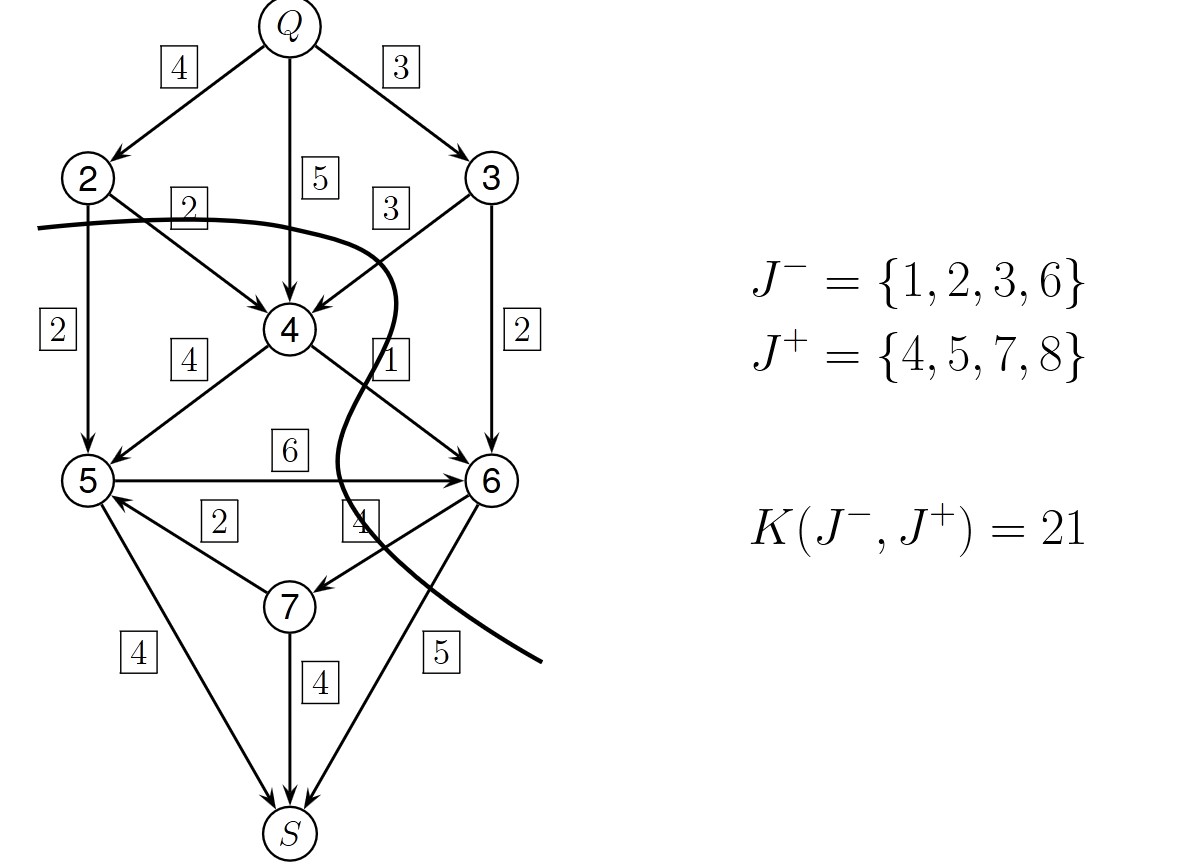
Definition
Let \(C\) be a capacity matrix. A cut \(J^-, J^+\) is a decomposition of the graph such that \(J^+ \cup J^- = \{1, \dots, n\}\) and \(J^+ \cap J^- = \emptyset\), with \(1 \in J^-\) and \(n \in J^+\). The capacity of a cut is:

$$ K(J^-, J^+) := \sum_{i \in J^-, j \in J^+} C_{ij} $$

In other words, to find the capacity of a cut, we sum the capacities of all edges that lie between \(J^-\) and \(J^+\).

Lemma
Let \(C\) be a capacity matrix. For every possible cut \(J^-, J^+\) and flow \(X\):

$$ W(X) \leq K(J^-, J^+) $$

This is the weak duality lemma. Maximizing the flow is the primal problem, while minimizing the capacity of the cut is the dual problem.

Next, we can state the strong duality lemma.

Lemma
The following is true:

$$ \max\{W(X) : X\} = \min\{K(J^+, J^-) : (J^+, J^-)\} $$

4.2 Game Theory

Game Situation: We have two players in a zero-sum game. Player 1 (\(P_1\)) has the option to choose any of the strategies \(a_1, \dots, a_n\), and Player 2 (\(P_2\)) can choose any of the alternative strategies \(b_1, \dots, b_n\). If \(P_1\) chooses the action \(a_i\) and \(P_2\) chooses the option \(b_j\), the resulting payout is \(a_{ij}\). Thus, the whole game and its payouts can be described in a matrix:

$$ A = \begin{pmatrix} a_{11} & a_{12} & \dots & a_{1n} \\ \vdots & \vdots & \ddots & \vdots \\ a_{m1} & \dots & \dots & a_{mn} \end{pmatrix} $$

For example, the game “rock-paper-scissors” can be written like this:

$$ A = \begin{pmatrix} 0 & 1 & -1 \\ -1 & 0 & 1 \\ 1 & -1 & 0 \end{pmatrix} $$

Game theory is interesting for modeling how economic players act in the long term. The central question is: How should a player act to be reasonable/optimal?

For this, players choose their strategies:

$$ x = (x_1, \dots, x_n)^T, \quad y = (y_1, \dots, y_n)^T $$

The strategies should sum to 1, i.e. \(\sum x_j = 1\), and each \(x_j\) gives the probability that Player 1 will choose strategy \(j\).

We call a strategy pure if \(x\) is a unit vector, meaning the player always chooses the same action. If this is not the case, the strategy is called mixed.

The expected payout for the game can be calculated as:

$$ \phi(x, y) := y^T A x $$

For Player 1 to act optimally, they should:

$$ \max_{x^T e = 1} y^T A x $$

But Player 2 should do the opposite. Thus, we have the following two optimization problems:

$$ \begin{aligned} & (P_1) \quad \min \max y^T A x, \quad x \geq 0, \, x^T e = 1 \\ & (P_2) \quad \max \min y^T A x, \quad y \geq 0, \, y^T e = 1 \end{aligned} $$

We can formalize this as a linear optimization problem:

$$ \begin{aligned} & (P^*_1) \quad \min x_0, \quad x \geq 0, \, x^T e = 1, \, A x \leq x_0 e \\ & (P^*_2) \quad \max y_0, \quad y \geq 0, \, y^T e = 1, \, A y \geq y_0 e \end{aligned} $$

These two problems are dual to each other, which is evident in the following lemma.

Lemma Main Theorem of Matrix Games
Let \(x^*, y^* \in \mathbb{R}\) with \(e^T x^* = 1\) and \(e^T y^* = 1\), then

$$ y^* A x^* = \min_x \max_y y^T A x = \max_y \min_x y^T A x =: v $$

The metric \(v\) is called the value of the matrix game.

Definition
A matrix game is called fair if the value is zero.

Lemma
If a matrix game \(A\) is skew-symmetric, i.e. \(A^T = -A\), then the value of the game is 0, and the game is fair.

Definition
A game described by the matrix \(A\) is called a saddle-point game if

$$ \min_j \max_i a_{ij} = \max_i \min_j a_{ij} $$

Lemma
Every saddle-point game has a solution consisting of pure strategies.

4.3 Set of Problems and Solutions

4.3.1 Matrix Game

Task: Rudy and Carla like to camp on a mountain. Rudy likes hills, and Carla likes valleys. The mountain on which they camp has \(n\) intersecting paths. They decide to camp at one of these intersections. As a compromise, Rudy is allowed to choose the first path, and Carla chooses the path that intersects with Rudy’s first choice. They further know the attitude of all the paths.

(a) Formulate this as a two-person matrix game, where Rudy tries to camp at a location as high as possible, and Carla tries to camp at a location as low as possible.
(b) What does “fair” mean in this context?
(c) Use the following table of attitudes to show that the game is a saddle-point game. Then, find the best strategies for the players and determine whether the game is fair or not.

$$ \begin{array}{|c|c|c|c|c|} \hline \text{} & \text{Path 1} & \text{Path 2} & \text{Path 3} & \text{Path 4} \\ \hline \text{Path 1} & 3500 & 1000 & 2500 & 500 \\ \text{Path 2} & 1000 & 1000 & 1500 & 2000 \\ \text{Path 3} & 2500 & 1500 & 2000 & 2000 \\ \text{Path 4} & 1500 & 1000 & 500 & 3000 \\ \hline \end{array} $$

Solution (a)

The payout matrix \(A = (a_{ik})\) represents the attitude of the intersections between the two paths. Carla is Player 1 (P1), and Rudy is Player 2 (P2).

Carla tries to minimize the attitude:

$$ \text{Maximize} \ \ x_0 \ \ \text{subject to} \ \ A x \leq x_0 e_n, \, x \geq 0 $$

Rudy tries to maximize the attitude:

$$ \text{Minimize} \ \ y_0 \ \ \text{subject to} \ \ A y \leq y_0 e_n, \, y \geq 0 $$

Solution (b)

Since the attitude values are greater than 0, we can’t use 0 as a criterion for determining whether the matrix game is fair. Instead, we should calculate the average attitude \(h\) and look at the modified payout matrix \(A - h e_n e_m^T\).

Solution (c)

To determine whether the matrix game is a saddle-point game, we need to check if the following condition is satisfied:

$$ \min_j \max_i a_{ij} = \max_i \min_j a_{ij} $$

We can see that:

$$ \begin{aligned} \min_j \max_i a_{ij} &= \min \{3500, 1500, 2500, 3000\} = 1500 \\ \max_i \min_j a_{ij} &= \max \{500, 1000, 1500, 500\} = 1500 \end{aligned} $$

Thus, the matrix game is a saddle-point game. Therefore, the optimal strategy is a pure strategy: Way 3 for Rudy and Way 2 for Carla.

Calculating the average attitude, we get \(h = 1687.5\). Hence, the game is not fair because Carla would win.

5. The Generic Simplex Method

The simplex algorithm is based on the idea that for linear optimization problems, it is enough to find an optimal corner to solve the problem. We can start at an arbitrary corner of the polyhedron and walk along its sides to the next corner, looking for a better value of the objective function. Since a polyhedron has a finite number of corners, the algorithm stops after a finite number of steps when it no longer finds a corner that improves the objective function.

The simplex algorithm takes as input a problem in the following canonical form:

$$ (P) \quad \text{Minimize} \ \ f(x) := c^T x \ \ \text{subject to} \ \ M = \{x \in \mathbb{R}^n : Ax = b, x \geq 0\} $$

If our optimization problem is not in this form, we need to transform it first by introducing slack variables to transform inequalities into equalities, and by introducing non-negative variables to ensure all variables are positive.

For example:

$$ \begin{aligned} & \text{Maximize } x_1 + 2x_2 \\ & \text{subject to:} \\ & x_1 + 2x_2 \leq 4, \\ & 2x_1 + x_2 \leq 3, \\ & x_2 \geq 1, \\ & x_j \geq 0, \quad j = 1, 2. \end{aligned} $$

This can be transformed into:

$$ \begin{aligned} & \text{Maximize } x_1 + 2x_2 \\ & \text{subject to:} \\ & x_1 + 2x_2 + x_3 = 4, \\ & 2x_1 + x_2 + x_4 = 3, \\ & x_2 + x_5 = 1, \\ & x_j \geq 0, \quad j = 1, \dots, 5. \end{aligned} $$

5.1 Idea of Simplex Algorithm on an Example

Maximize \( 20x_1 + 60x_2 \) under the constraints:

$$ \begin{pmatrix} 1 & 1 \\ 5 & 10 \\ 2 & 10 \end{pmatrix} \begin{pmatrix} x_1 \\ x_2 \end{pmatrix} \leq \begin{pmatrix} 120 \\ 700 \\ 520 \end{pmatrix}, \quad x_1, x_2 \geq 0 $$

The first step is to bring the problem into the desired canonical form by introducing slack variables. Furthermore, we need to minimize \( - 20x_1 - 60x_2 \) under the following constraints:

$$ \begin{pmatrix} 1 & 1 & 1 & 0 & 0 \\ 5 & 10 & 0 & 1 & 0 \\ 2 & 10 & 0 & 0 & 1 \end{pmatrix} \cdot \begin{pmatrix} x_1 \\ x_2 \\ x_3 \\ x_4 \\ x_5 \end{pmatrix} \ = \ \begin{pmatrix} 120 \\ 700 \\ 520 \end{pmatrix} $$

This system of equations is in the form for Gaussian elimination. The variables \(x_1, x_2\) are free variables, while \(x_3, x_4, x_5\) are dependent variables. By setting the free variables to zero, we obtain the basic solution \( Z = (0, 0, 120, 700, 520)^T \), which is the first corner of our polyhedron.

We can now represent this in the form of a table, where the first row contains the function we want to minimize, followed by the constraints. The pivot entry is the one from which we perform the Gaussian elimination:

$$ \begin{array}{ccccc|c} -20 & -60 & 0 & 0 & 0 & 0 \\ \hline 1 & 1 & 1 & 0 & 0 & 120 \\ 5 & 10 & 0 & 1 & 0 & 700 \\ 2 & \fbox{10} & 0 & 0 & 1 & 520 \\ \end{array} $$

Since \( b \geq 0 \), our basis solution is valid. We can continue to the next table through Gaussian elimination:

$$ \begin{array}{ccccc|c} -8 & 0 & 0 & 0 & 6 & 3120 \\ \hline 4/5 & 0 & 1 & 0 & 1/-10 & 68 \\ 3 & 0 & 0 & 1 & -1 & 180 \\ 1/5 & 1 & 0 & 0 & 1/10 & 52 \\ \end{array} $$

Now \( x_1, x_5 \) are free variables, and \( x_2, x_3, x_4 \) are dependent. The associated basic solution, obtained by setting the free variables to zero, is \( Z = (0, 52, 68, 180, 0)^T \).

Interlude

If we had used \( a_{12} \) as the pivot instead of \( a_{32} \), we would have gotten the following matrix:

$$ \begin{array}{ccccc|c} 40 & 0 & 60 & 0 & 0 & 60 \cdot 120 \\ \hline 1 & 1 & 1 & 0 & 0 & 120 \\ -5 & 0 & -10 & 1 & 0 & -500 \\ -8 & 0 & -10 & 0 & 1 & -680 \\ \end{array} $$

And we would have the basis solution \( (0, 120, 0, -500, -680)^T \). This is not a valid solution, since some components are negative.

Continuing the example, we choose the pivot entry that is in the first column with a negative entry, and from the column where \( \frac{b_r}{a_{rs}} \) is minimal:

$$ \begin{array}{ccccc|c} −8 & 0 & 0 & 0 & 6 & 3120 \\ \hline 4/5 & 0 & 1 & 0 & −1/10 & 68 \\ \fbox{3} & 0 & 0 & 1 & −1 & 180 \\ 1/5 & 1 & 0 & 0 & 1/10 & 52 \end{array} $$

After performing the necessary Gaussian elimination steps:

$$ \begin{array}{ccccc|c} 0 & 0 & 0 & 8/3 & 10/3 & 3600 \\ \hline 0 & 0 & 1 & −4/15 & 1/6 & 20 \\ 1 & 0 & 0 & 1/3 & −1/3 & 60 \\ 0 & 1 & 0 & −1/15 & 1/6 & 40 \end{array} $$

The basic solution at this point is \( x^* = (60, 40, 20, 0, 0)^T \) with \( f(x^*) = -3600 \). The first row of the table represents the cost vector. Since all entries in the cost vector are now positive, the simplex algorithm is finished, and we have found the optimal solution.

We can now disregard the slack variables \( x_3, x_4, x_5 \) and have the optimal solution vector \( (60, 40)^T \).

The process you just saw is called Phase 2 of the simplex algorithm, where, starting from a basis solution, the algorithm iterates through the corners of the polyhedron to find the optimal solution. Phase 1 is used when we need to transform our problem into canonical form so that it can be used for Phase 2. Phase 1 is necessary if the problem does not yet have a basis solution.

5.2 The Simplex Algorithm

The simplex algorithm consists of two phases:

5.2.1 Phase 1

The goal of Phase 1 is to construct a basic solution \( z \) for the system \( Ax = b \). It does this by solving a helper problem:

$$ \min e^T(b - Ax) $$

on the feasible region

$$ M_H = \{x \in \mathbb{R}^n : Ax \leq b\} $$

The simplex tableau for Phase 1 is represented as follows:

$$ \begin{array}{cccccc|c} -\sum a_{i1} & \dots & -\sum a_{in} & 0 & \dots & 0 & -\sum b_i \\ \hline c_1 & \dots & c_n & 0 & \dots & 0 & 0 \\ \hline a_{11} & \dots & a_{1n} & 1 & \dots & 0 & b_1 \\ \vdots & & \vdots & \vdots & & \vdots & \vdots \\ a_{m1} & \dots & a_{mn} & 0 & \dots & 1 & b_m \\ \end{array} $$

After solving the Phase 1 problem, we proceed with Phase 2 of the simplex algorithm, which continues until the first row is entirely positive. There are two possible outcomes:

1. Case 1: \( e^T(b - Az) = 0 \) – In this case, a valid basic solution has been found, and we can remove the row and columns added in Phase 1 and proceed with Phase 2.

2. Case 2: \( e^T(b - Az) > 0 \) – This means that the feasible region \( M_H \) is empty, and the problem is invalid (no solution exists).

5.2.2 Phase 2

After Phase 1, we proceed with Phase 2. At this stage, the tableau is as follows:

$$ \begin{array}{c|c} c^T & 0 \\ \hline A & b \end{array} $$

In Phase 2, we iteratively construct a new basic solution, improving the objective function value (the top right corner) at each step, until the minimum is reached.

1. If \( c \ge 0 \): The current basic solution \( z \) is optimal, and the value in the top right corner of the tableau represents the optimal value of the objective function.

2. Pivot Rule (Bland’s Rule):

   • Pivot column: Choose \( s = \min\{n : c_n \leq 0\} \), i.e., the first column where the entry is negative.
   • If \( a_{rs} \leq 0 \) for all \( r \), then the problem has an unbounded objective value and the minimum is \( -\infty \).
   • Pivot row: Choose the row \( r \) where \( \frac{b_r}{a_{rs}} \) is minimal, subject to \( a_{rs} > 0 \).
   • The pivot element is \( a_{rs} \).

3. Perform Gaussian elimination to make the pivot element \( a_{rs} = 1 \) and all other elements in the pivot column \( s \) equal to zero.

4. Determine the new basic solution \( z \) and the updated objective function value.

5. Return to step 1 and repeat until the solution converges.

5.3 Interpretation of the Simplex Algorithm

The simplex algorithm has a very insightful geometric interpretation, particularly in the context of two-dimensional optimization problems.

5.4 Set of Problems and Solutions

5.4.1 Basic Example: Phase 2

Task: Determine the maximum of the objective function \(Z(x,y) = -x + 3y\) under the constraints:

\[ x + y \leq 5, \quad x - y \geq -3, \quad x \leq 2, \quad x, y \geq 0 \]

Solution

Step 1: Transform the problem into canonical form.

We first express the objective function as a minimization problem:

\[ \max \quad -x + 3y \quad \text{becomes} \quad \min \quad x - 3y \]

Now, we add slack variables to convert inequalities into equalities:

\[ x + y + x_3 = 5, \quad -x + y + x_4 = 3, \quad x + x_5 = 2 \]

Thus, the problem becomes:

\[ \min \quad x_1 - 3x_2 \]

subject to:

\[ x_1 + x_2 + x_3 = 5, \quad -x_1 + x_2 + x_4 = 3, \quad x_1 + x_5 = 2 \]

with \(x_1, x_2, x_3, x_4, x_5 \geq 0\).

Step 2: Set up the initial simplex tableau.

The initial tableau looks like this:

\[ \begin{array}{ccccc|c} x_1 & x_2 & x_3 & x_4 & x_5 & b \\ \hline 1 & -3 & 0 & 0 & 0 & 0 \\ \hline 1 & 1 & 1 & 0 & 0 & 5 \\ -1 & 1 & 0 & 1 & 0 & 3 \\ 1 & 0 & 0 & 0 & 1 & 2 \\ \end{array} \]

Step 3: Find the pivot element using Bland’s Rule.

• The first negative column is the second column (corresponding to \(x_2\)).
• Compute \( \min \left\{ \frac{b_k}{a_{ks}} : a_{ks} > 0 \right\} \) for the second column: \[ \frac{5}{1}, \quad \frac{3}{1}, \quad \frac{2}{1} \] The lowest ratio is 2, corresponding to the third row.

Step 4: Perform the first iteration (Gaussian elimination) to make all other entries in the pivot column (second column) zero.

\[ \begin{array}{ccccc|c} x_1 & x_2 & x_3 & x_4 & x_5 & b \\ \hline -2 & 0 & 0 & 3 & 0 & 9 \\ \hline 2 & 0 & 1 & -1 & 0 & 2 \\ -1 & 1 & 0 & 1 & 0 & 3 \\ 1 & 0 & 0 & 0 & 1 & 2 \\ \end{array} \]

Step 5: Find the next pivot element.

• The first negative entry is in the first column, and the lowest ratio is \( \frac{9}{2} = 4.5 \), which corresponds to the first row.

Step 6: Perform the second iteration of Gaussian elimination.

\[ \begin{array}{ccccc|c} x_1 & x_2 & x_3 & x_4 & x_5 & b \\ \hline 0 & 0 & 0 & 1 & 2 & 11 \\ \hline 1 & 0 & \frac{1}{2} & -\frac{1}{2} & 0 & 1 \\ 0 & 1 & \frac{1}{2} & \frac{1}{2} & 0 & 4 \\ 0 & 0 & -\frac{1}{2} & \frac{1}{2} & 1 & 1 \\ \end{array} \]

Step 7: Check the top row.

Since all the entries in the top row are now non-negative, the algorithm terminates. The optimal solution is \(x_1 = 1\), \(x_2 = 4\), and the maximum value of \(Z\) is \(Z = 11\).

Thus, the optimal solution is \(x = 1\), \(y = 4\), with \(Z = 11\).

5.4.2 Basic Example: Phase 2

Task: A Truck can transport up to 20 tonnes of freight with 12m³ space, and it can be loaded with two goods \(G_1, G_2\). Each good has 8 units in stock.

\[ \begin{array}{|c|c|c|} \hline & G_1 & G_2 \\ \hline \text{Weight (Tonnes)} & 2 & 3 \\ \text{Space (m}^3\text{)} & 2 & 1 \\ \text{Worth (in 10,000€)} & 3 & 2 \\ \hline \end{array} \]

How many units of each good should the truck be loaded with, to maximize the freight?

Solution

1. Bring the problem in canonical form:

\[ \begin{aligned} \max \quad & 3 G_1 + 2 G_2 \\ \text{subject to} \quad & 2 G_1 + 3 G_2 \leq 20, \\ & 2 G_1 + 1 G_2 \leq 12, \\ & G_1 \leq 8, \\ & G_2 \leq 8, \\ & G_1, G_2 \geq 0. \end{aligned} \]

2. Add slack variables and transform from maximization to minimization:

\[ \begin{aligned} \max \quad & -3 G_1 -2 G_2 \\ \text{subject to} \quad & 2 G_1 + 3 G_2 + x_1 = 20, \\ & 2 G_1 + 1 G_2 + x_2 = 12, \\ & G_1 + x_3 = 8, \\ & G_2 + x_4 = 8, \\ & x_1, x_2 \geq 0. \end{aligned} \]

3. Write the problem in the form of a table:

\[ \begin{array}{cccccc|c} G_1 & G_2 & x_1 & x_2 & x_3 & x_4 & b \\ \hline -3 & -2 & 0 & 0 & 0 & 0 & 0 \\ \hline 2 & 3 & 1 & 0 & 0 & 0 & 20 \\ 2 & 1 & 0 & 1 & 0 & 0 & 12 \\ 1 & 0 & 0 & 0 & 1 & 0 & 8 \\ 0 & 1 & 0 & 0 & 0 & 1 & 8 \\ \end{array} \]

4. Find the pivot with Bland’s rule:
   • The first negative column is the first column.
   • The lowest division is in the second row.

\[ \begin{array}{cccccc|c} G_1 & G_2 & x_1 & x_2 & x_3 & x_4 & b \\ \hline -3 & -2 & 0 & 0 & 0 & 0 & 0 \\ \hline 2 & 3 & 1 & 0 & 0 & 0 & 20 \\ \fbox{2} & 1 & 0 & 1 & 0 & 0 & 12 \\ 1 & 0 & 0 & 0 & 1 & 0 & 8 \\ 0 & 1 & 0 & 0 & 0 & 1 & 8 \\ \end{array} \]

5. First Iteration:

\[ \begin{array}{cccccc|c} G_1 & G_2 & x_1 & x_2 & x_3 & x_4 & b \\ \hline 0 & -0.5 & 0 & 1.5 & 0 & 0 & 18 \\ \hline 0 & 2 & 1 & -1 & 0 & 0 & 8 \\ 1 & 0.5 & 0 & 0.5 & 0 & 0 & 6 \\ 0 & -0.5 & 0 & -0.5 & 1 & 0 & 2 \\ 0 & 1 & 0 & 0 & 0 & 1 & 8 \\ \end{array} \]

6. Find the pivot with Bland’s rule:
   • The first negative column is the second column.
   • The lowest division is in the first row.

\[ \begin{array}{cccccc|c} G_1 & G_2 & x_1 & x_2 & x_3 & x_4 & b \\ \hline 0 & -0.5 & 0 & 1.5 & 0 & 0 & 18 \\ \hline 0 & \fbox{2} & 1 & -1 & 0 & 0 & 8 \\ 1 & 0.5 & 0 & 0.5 & 0 & 0 & 6 \\ 0 & -0.5 & 0 & -0.5 & 1 & 0 & 2 \\ 0 & 1 & 0 & 0 & 0 & 1 & 8 \\ \end{array} \]

7. Second Iteration:

\[ \begin{array}{cccccc|c} G_1 & G_2 & x_1 & x_2 & x_3 & x_4 & b \\ \hline 0 & 0 & \frac{1}{4} & \frac{5}{4} & 0 & 0 & 20 \\ \hline 0 & 1 & \frac{1}{2} & -\frac{1}{2} & 0 & 0 & 4 \\ 1 & 0 & -\frac{1}{4} & \frac{3}{4} & 0 & 0 & 4 \\ 0 & 0 & \frac{1}{4} & -\frac{3}{4} & 1 & 0 & 4 \\ 0 & 0 & -\frac{1}{2} & \frac{1}{2} & 0 & 1 & 4 \\ \end{array} \]

8. Optimal Solution:

The top row is completely positive, indicating that we have found the optimal solution, which is \(z = 20\) with \(G_1 = 4\), \(G_2 = 4\).

5.4.3 Intermediate Example: Phase 2

Task: Let \(\alpha, \beta \in \mathbb{R}\). Solve the following problem with the simplex algorithm:

\[ \begin{aligned} \text{Maximize} & \quad f(x) = \alpha x_1 + \beta x_2 \\ \text{subject to} \quad & x_1 \geq 0, \, x_2 \geq 0, \, x_1 - x_2 \leq 10 \end{aligned} \]

Solution

Case 1 \(\beta > 0\): Then the problem is unrestricted, since we can set \(\alpha = 0\) and \(x_2 \to \infty\). We only need to fulfill the restriction \(x_1 - x_2 \leq 10\), which can be done by also letting \(x_2 \to \infty\).

Case 2 \(\beta \leq 0\): We need to add a slack variable \(x_3\) for the restriction \(x_1 - x_2 \leq 10\), and then we can write the problem in table form:

\[ \begin{array}{ccc|c} x_1 & x_2 & x_3 & b \\ \hline -\alpha & -\beta & 0 & 0 \\ \hline 1 & -1 & 1 & 10 \end{array} \]

We now need to calculate the pivot again using Bland’s rule:

\[ \begin{array}{ccc|c} x_1 & x_2 & x_3 & b \\ \hline -\alpha & -\beta & 0 & 0 \\ \hline \fbox{1} & -1 & 1 & 10 \end{array} \]

It now depends on the sign of \(\alpha\) how to proceed. If \(\alpha \leq 0\), then all our values in the first row are positive, and we stop the simplex algorithm, meaning we have already reached our optimal value \(f(0, 0) = 0\).

Otherwise, we can continue:

\[ \begin{array}{ccc|c} x_1 & x_2 & x_3 & b \\ \hline 0 & -\beta - \alpha & 0 & 10 \alpha \\ \hline 1 & -1 & 1 & 10 \end{array} \]

If \(-\beta - \alpha \geq 0\), then the first row is positive, and we have reached the optimum value with \(f(10) = 10 \alpha\).

Otherwise, if \(-\beta - \alpha \le 0\), then we need to continue and calculate the next pivot, but the only entry in the second row is \(-1 \leq 0\), thus we can’t continue. This means our problem is unrestricted, i.e., \(\max f(x) = \infty\).

5.4.4 Basic Example: Phase 1

Task: Minimize \(- x_1 + 2x_2 + 3x_3\) under the restrictions:

\[ \begin{aligned} x_1 + 3x_2 - 2x_3 &\leq 10 \\ 3x_1 - 2x_2 - 3x_3 &\leq -5 \\ 4x_1 - 2x_3 &= 4 \\ x_1, x_2 &\geq 0 \end{aligned} \]

Solution

The first step is to bring the problem into its canonical form, by replacing \(x_3\) which is not positive by two positive variables \(x_3 - x_4\) with \(x_3, x_4 \geq 0\). Furthermore, we need to introduce slack variables \(x_5, x_6\) for the first two restrictions. We further multiply the second equality by \(-1\), which gives us the following problem:

\[ \begin{aligned} \min \quad & -x_1 + 2x_2 + 3x_3 - 3x_4 \\ \text{subject to:} \quad & x_1 + 3x_2 - 2x_3 + 2x_4 + x_5 = 10, \\ & -3x_1 + 2x_2 + 3x_3 - 3x_4 - x_6 = 5, \\ & 4x_1 - 2x_2 = 4, \\ & x_j \geq 0 \quad \text{for } j = 1, 2, 3, 4, 5, 6. \end{aligned} \]

We can write this in tabular form:

\[ \begin{array}{cccccc|c} x_1 & x_2 & x_3 & x_4 & x_5 & x_6 & b \\ \hline -1 & 2 & 3 & -3 & 0 & 0 & 0 \\ \hline 1 & 3 & -2 & 2 & 1 & 0 & 10 \\ -3 & 2 & 3 & -3 & 0 & -1 & 5 \\ 4 & -2 & 0 & 0 & 0 & 0 & 4 \\ \end{array} \]

But we have a problem in the second row, the entry for the variable \(x_6\) is negative, but in our restriction set we assumed \(x_6 \geq 0\) as required by the simplex algorithm (the simplex algorithm uses the canonical form which has the prerequisite that \(x_j \geq 0\)).

Thus, we first need to transform our problem using Phase 1 of the simplex algorithm and get a first basis solution on which we can then iterate using Phase 2.

Since the first equation is already in the correct form, we need to apply the transformation only on the bottom two equalities. So, first we need to add a new column with entries that are the sum of entries for each column multiplied by \(-1\). For example, the first entry in our new row will be \((-3) + 4 = 1 \implies (-1) \cdot 1 = -1\), and remember we only add up the last two rows. We further add two new rows with unit vectors in them.

We also calculate the pivot and mark it:

\[ \begin{array}{cccccc|c} -1 & 0 & -3 & 3 & 0 & 1 & 0 & 0 & -9 \\ \hline -1 & 2 & 3 & -3 & 0 & 0 & 0 & 0 & 0 \\ \hline 1 & 3 & -2 & 2 & 1 & 0 & 0 & 0 & 10 \\ -3 & 2 & \fbox{3} & -3 & 0 & -1 & 1 & 0 & 5 \\ 4 & -2 & 0 & 0 & 0 & 0 & 0 & 1 & 4 \\ \end{array} \]

Next, we perform the necessary steps to finalize Phase 1:

\[ \begin{array}{cccccc|c} -4 & 2 & 0 & 0 & 0 & 0 & 1 & 0 & -4 \\ \hline 2 & 0 & 0 & 0 & 0 & 1 & -1 & 0 & -5 \\ \hline -1 & \frac{13}{3} & 0 & 0 & 1 & -\frac{2}{3} & \frac{2}{3} & 0 & \frac{40}{3} \\ -1 & \frac{2}{3} & 1 & -1 & 0 & -\frac{1}{3} & \frac{1}{3} & 0 & \frac{5}{3} \\ \fbox{4} & -2 & 0 & 0 & 0 & 0 & 0 & 1 & 4 \\ \end{array} \]\[ \begin{array}{cccccc|c} 0 & 0 & 0 & 0 & 0 & 0 & 1 & 1 & 0 \\ \hline 0 & 1 & 0 & 0 & 0 & 1 & -1 & -\frac{1}{2} & -7 \\ \hline 0 & \frac{23}{6} & 0 & 0 & 1 & -\frac{2}{3} & \frac{2}{3} & \frac{1}{4} & \frac{43}{3} \\ 0 & \frac{1}{6} & 1 & -1 & 0 & -\frac{1}{3} & \frac{1}{3} & \frac{1}{4} & \frac{8}{3} \\ 1 & -\frac{1}{2} & 0 & 0 & 0 & 0 & 0 & \frac{1}{4} & 1 \\ \end{array} \]

Now that the first row has zeros in the positions we want, we are finished and can move to Phase 2. Our basis solution is \(z = (1, 0, 8/3, 0, 43/3, 0, 0, 0)\).

To move on to Phase 2, we can remove the first row and the last two columns before the \(b\)-column:

\[ \begin{array}{cccccc|c} 0 & 1 & 0 & 0 & 0 & 1 & -7 \\ \hline 0 & \frac{23}{6} & 0 & 0 & 1 & -\frac{2}{3} & \frac{43}{3} \\ 0 & \frac{1}{6} & 1 & -1 & 0 & -\frac{1}{3} & \frac{8}{3} \\ 1 & -\frac{1}{2} & 0 & 0 & 0 & 0 & 1 \\ \end{array} \]

As we see, Phase 2 is already finished since the first row has only positive values. The solution is \(x^* = (1, 0, 8/3), f(x^*) = 7\).

5.4.5 Intermediate Example: Phase 1

Task: Minimize \(x_1 - x_2\) under the following constraints: \(x_1 + x_2 \leq 3\), \(x_1 + 2x_2 \geq 1\), \(x_1 \geq 0\).

Solution

First, write the problem in its canonical form. We need to add slack variables for the two inequalities and replace \(x_2 := x_2 - x_3\) so that all variables are positive.

$$ \begin{aligned} \min \quad & x_1 - x_2 - x_3 \\ \text{subject to} \quad & x_1 + x_2 - x_3 + x_4 = 3, \\ & x_1 + 2x_2 - x_5 = 1, \\ & x_1, x_2, x_3, x_4, x_5 \geq 0. \end{aligned} $$

Since we have \(- x_5\), we have a negative slack variable (remember, the rows of our slack variables need to be unit vectors), thus we need to start with Phase 1. For Phase 1, the table would look like this:

$$ \begin{array}{ccccc|c} x_1 & x_2 & x_3 & x_4 & x_5 & b \\ \hline 1 & -1 & -1 & 0 & 0 & 0 \\ \hline 1 & 1 & -1 & 1 & 0 & 3 \\ 1 & 2 & 0 & 0 & -1 & 1 \\ \end{array} $$

We create our Phase 1 table by adding a new row, whose entries are the sum of its columns multiplied by \(-1\). We furthermore add two columns with unit vectors. The pivot should be calculated and marked.

$$ \begin{array}{ccccc:c:c|c} x_1 & x_2 & x_3 & x_4 & x_5 & x_6 & x_7 & b \\ \hline -2 & -3 & 3 & -1 & 1 & 0 & 0 & -4 \\ \hline 1 & -1 & 1 & 0 & 0 & 0 & 0 & 0 \\ \hline 1 & 1 & -1 & 1 & 0 & 1 & 0 & 3 \\ \fbox{1} & 2 & -2 & 0 & -1 & 0 & 1 & 1 \\ \end{array} $$

Through the first iteration, we get:

$$ \begin{array}{ccccc:c:c|c} x_1 & x_2 & x_3 & x_4 & x_5 & x_6 & x_7 & b \\ \hline 0 & 1 & -1 & -1 & -1 & 0 & 2 & -2 \\ \hline 0 & -3 & 3 & 0 & 1 & 0 & -1 & -1 \\ \hline 0 & -1 & \fbox{1} & 1 & 1 & 1 & -1 & 2 \\ 1 & 2 & -2 & 0 & -1 & 0 & 1 & 1 \\ \end{array} $$

And:

$$ \begin{array}{ccccc:c:c|c} x_1 & x_2 & x_3 & x_4 & x_5 & x_6 & x_7 & b \\ \hline 0 & 0 & 0 & 0 & 0 & 1 & 1 & -1 \\ \hline 0 & 0 & 0 & -3 & -2 & -3 & 2 & -7 \\ \hline 0 & -1 & 1 & 1 & 1 & 1 & -1 & 2 \\ 1 & 0 & 0 & 2 & 1 & 2 & -1 & 5 \\ \end{array} $$

Since we now have zeros in the first row where we want them, we have finished Phase 1 and can continue to Phase 2. To get the table for Phase 2, we remove the last two columns and the first row of the table and calculate the pivot again.

$$ \begin{array}{ccccc|c} x_1 & x_2 & x_3 & x_4 & x_5 & b \\ \hline 0 & 0 & 0 & -3 & -2 & -7 \\ \hline 0 & -1 & 1 & \fbox{1} & 1 & 2 \\ 1 & 0 & 0 & 2 & 1 & 5 \\ \end{array} $$

We get through the first iteration of Phase 2:

$$ \begin{array}{ccccc|c} x_1 & x_2 & x_3 & x_4 & x_5 & b \\ \hline 0 & -3 & 3 & 0 & 1 & -1 \\ \hline 0 & -1 & 1 & 1 & 1 & 2 \\ 1 & \fbox{2} & -2 & 0 & -1 & 1 \\ \end{array} $$

Then:

$$ \begin{array}{ccccc|c} x_1 & x_2 & x_3 & x_4 & x_5 & b \\ \hline \frac{3}{2} & 0 & 0 & 0 & -\frac{1}{2} & \frac{1}{2} \\ \hline \frac{1}{2} & 0 & 0 & 1 & \fbox{\(\frac{1}{2}\)} & \frac{5}{2} \\ \frac{1}{2} & 1 & -1 & 0 & -\frac{1}{2} & \frac{1}{2} \\ \end{array} $$

Finally, the last step:

$$ \begin{array}{ccccc|c} x_1 & x_2 & x_3 & x_4 & x_5 & b \\ \hline 2 & 0 & 0 & 1 & 0 & 3 \\ \hline 1 & 0 & 0 & 2 & 1 & 5 \\ 1 & 1 & -1 & 1 & 0 & 3 \\ \end{array} $$

Hence, we have reached our optimal solution with \(x^* = (x_1, x_2, x_3) = (0, 3, 0)\). Remember, you get the solution by checking which columns are unit vectors; non-unit vector columns mean they have the value 0. This is the same as \(x^* = (x_1, x_2) = (0, 3 - 0) = (0, 3)\) and \(f(x^*) = -3\).

5.4.6 Advanced Example: Phase 1

Task: We have the following system of equations with \( \beta \in \mathbb{R}\):

$$ \begin{align*} \begin{bmatrix} 1 & 4 & 2 \\ -1 & 2 & -4 \end{bmatrix} \begin{bmatrix} x_1 \\ x_2 \\ x_3 \end{bmatrix} &= \begin{bmatrix} 2 \\ \beta \end{bmatrix} \end{align*} $$

Check for all \(\beta \geq 0\) with the help of Phase 1 of the simplex algorithm if the system of equations has a non-negative solution.

Solution

This problem is the same as asking whether \(M = \{Ax = b, x \geq 0\}\) is the empty set or not. This means asking whether a linear program is valid/feasible or not. We can solve this using Phase 1 of the simplex algorithm.

First, we create the Phase 1 table:

$$ \begin{array}{ccc:c:c|c} 0 & -6 & 2 & 0 & 0 & -2 -\beta \\ \hline 1 & 4 & 2 & 1 & 0 & 2 & \\ \hline -1 & 2 & -4 & 0 & 1 & \beta \\ \end{array} $$

The pivot will be in the second column. However, it depends on the value of \(\beta\) whether it will be the first row or the second row.

Case 1 \(\beta \geq 1\): Then 4 is the pivot, and we get the table:

$$ \begin{array}{ccc:c:c|c} \frac{3}{2} & 0 & 1 & \frac{3}{2} & 0 & 1 -\beta \\ \hline \frac{1}{4} & 1 & \frac{1}{2} & \frac{1}{4} & 0 & \frac{1}{2} & \\ \hline -\frac{3}{2} & 0 & -5 & -\frac{1}{2} & 1 & \beta - 1 \\ \end{array} $$

If \(\beta = 1\), then Phase 1 is finished as the cost vector (the first row of the table) is positive, with \(\min f = 0\). If \(\beta > 1\), then \(M = \emptyset\).

Case 2 \(0 \leq \beta \leq 1\): Then 2 is the pivot, and we get the table:

$$ \begin{array}{ccc:c:c|c} -3 & 0 & -10 & 0 & 3 & -2 + 2 \beta \\ \hline \fbox{3} & 0 & 10 & 1 & -2 & 2 - 2 \beta & \\ \hline -\frac{1}{2} & 1 & -2 & 0 & \frac{1}{2} & \frac{\beta}{2} \\ \end{array} $$

Then:

$$ \begin{array}{ccc:c:c|c} 0 & 0 & 0 & 1 & 1 & 0 \\ \hline 1 & 0 & \frac{10}{3} & \frac{1}{3} & -\frac{2}{3} & \frac{2}{3} - \frac{2}{3} \beta & \\ \hline 0 & 1 & -\frac{1}{3} & \frac{1}{6} & \frac{1}{6} & \frac{1}{3} + \frac{1}{6} \beta \\ \end{array} $$

With this, Phase 1 is finished, and the problem has a solution for \( 0 \leq \beta \leq 1\).

5.4.7 Simplex, Feasibility, and Solvability

Task: We have the following linear program:

$$ (P) \quad \text{Minimize} \ \ c^T x \ \ \text{under} \ \ Ax = b, \ x \geq 0, \ b \geq 0 $$

Furthermore, we have the helper problem:

$$ (P') \quad \text{Minimize} \ \ c^T x + \alpha e^T z \ \ \text{under} \ \ Ax + z = b, \ x \geq 0, \ b \geq 0, \ z \geq 0 $$

Show that:

(a) There is an immediate basic solution for (P’).
(b) If \((x^*, z^*)\) is a solution of (P’) with \(z^* = 0\), then \(x^*\) is a solution for (P).

Solution (a)

We can write (P’) in its canonical form:

$$ \begin{bmatrix} A & I \end{bmatrix} \begin{bmatrix} x \\ z \end{bmatrix} = b $$

Since \(b \geq 0\) according to the task description, we have the basic solution \((x, z) = (0, b)\).

Solution (b)

We are given our solution \((x^*, z^*)^T\) of problem (P’). Since \(z^* = 0\), the constraints of (P’) are \(Ax^* = b\), \(x^* \geq 0\). This means that \(x^*\) is a feasible point (a possible solution, since it fulfills the constraints) of (P).

It remains to show that \(x^*\) is the optimal solution.

Since \((x^*, z^*)\) is optimal for (P’):

$$ c^T x^* = c^T x^* + \alpha e^T z^* \leq c^T x + \alpha e^T 0 = c^T x $$

This means that \(x^*\) is optimal for (P).

6. Convex Optimization

Until now, we have only seen linear optimization problems, with linear objective functions and linear constraints. We now want to explore another important family of functions that we want to optimize: convex functions.

6.1 Convex Functions

Definition
We call a set \(M \subset \mathbb{R}^n\) convex if for \(x, y \in M\) and \(\lambda \in [0,1]\), the following holds: \((1 - \lambda)x + \lambda y \in M\).

In other words, we say that a set is convex if we have two points \(a, b\), and their interval \([a, b]\) is also in the set. In convex optimization problems, both the domain of the definition and the target area are convex sets.

Definition
Let \(D \subset \mathbb{R}^n\) be convex.
a) A function \(f : D \to \mathbb{R}\) is called convex if for all \(x, y \in D\) and \(\lambda \in [0,1]\), the following applies:

$$ f (\lambda x + (1 - \lambda) y) \leq \lambda f(x) + (1 - \lambda) f(y) $$

b) A function \(f : D \to \mathbb{R}\) is called strictly convex if for all \(x, y \in D\) with \(x \neq y\) and \(\lambda \in (0, 1)\), the following applies:

$$ f (\lambda x + (1 - \lambda) y) < \lambda f(x) + (1 - \lambda) f(y) $$

c) A function \(f : D \to \mathbb{R}\) is called steadily convex if there exists \(c_0 > 0\) such that for all \(x, y \in D\) and \(\lambda \in [0, 1]\), the following applies:

$$ f (\lambda x + (1 - \lambda) y) + c_0 \lambda (1 - \lambda) || x - y ||^2 \leq \lambda f(x) + (1 - \lambda) f(y) $$

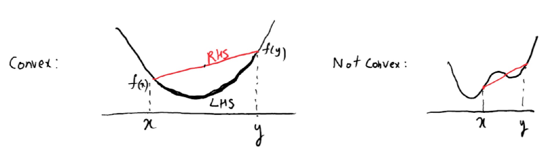
Convex functions are defined analogously to convex sets. We say a function is convex when, for any two points, we can draw a line between them that is above the function.

Example

a) The function \(f(x) = c^T x, x \in \mathbb{R}^n\) is convex, but not strictly convex.

b) \(f(x) = \frac{1}{1 + x}, x \geq 0\) is strictly convex, but not steadily convex.

c) Let \(Q \in \mathbb{R}^{n \times n}\) be symmetric and positive definite, then \(f(x) = x^T Qx + c^T x\) is convex.

We can define the gradient \( \nabla f (x)\), which gives us the rate of change (first derivative) in all directions. We also have the Hessian matrix \( \nabla^2 f(x)\), which gives the second rate of change (i.e., the second derivative) of this function.

Lemma
Let \( D \subset \mathbb{R}^n \) be open and convex, then the following holds:

a) \(f\) is steadily convex on \(D\), if one of the following equivalent conditions holds:

• There exists \(c_0 \geq 0\) such that \(f(x) - f(y) \geq \nabla f(y)^T (x - y) + c_0 ||x - y||^2\)
• There exists \(c_0 \geq 0\) such that \(z^T \nabla^2 f(x) z \geq 2 c_0 ||z||^2\)

b) \(f\) is strictly convex, when in (a) we can replace \(c_0 = 0\) and “\(\leq\)” with “\(<\)” for \(x \neq y, z \neq 0\).

c) \(f\) is convex, when in (a) we can replace \(c_0 = 0\).

This means that if we want, for example, to show that a certain function is convex, we can show that its second derivative is always positive.

6.2 Existence and Unambiguity

For linear optimization problems, it was sufficient for \(M \neq \emptyset\) and \(\inf(P) \geq -\infty\) for a solution to exist, i.e., for the problem to have a solution.

In general, this is not true for convex optimization problems.

Example

Let’s look at the function

$$ f(x) = \frac{1}{x} $$

for which \(\inf \ f(x) = 0\), but \(f(x) > 0\), meaning we can never reach the optimal solution.

Thus, we need additional conditions and prerequisites for our convex optimization problem to be solvable.

We now look at the general convex problem:

$$ (P) \quad \min f(x), \quad M = \{x \in K : g(x) \leq 0, Ax = b\} $$

where \(K \subset \mathbb{R}^n\) is a convex set, and \(f, g\) are convex functions.

In optimization theory, we differentiate between local minima (the lowest point in a subset of the landscape) and global minima (the lowest point in the overall landscape). But for convex functions, they are one and the same.

Lemma
All local minima of a convex function are also global minima. The set of minima is convex.

Lemma
(P) has a solution if \(M \neq \emptyset\), \(\inf(P) \leq -\infty\), and \(\Lambda = \{(f(x) + r, g(x) + z, Ax - b) \in \mathbb{R} \times \mathbb{R}^p \times \mathbb{R}^m : r \geq 0, z \geq 0, x \in K\}\) is closed.

Lemma
If \(M \neq \emptyset\) and \(f\) is strictly convex, then (P) has at most one solution.

Lemma
If \(M \neq \emptyset\) and \(f\) is steadily convex, then (P) has exactly one unambiguous solution.

6.3 The Dual Problem and Duality Lemmas

Let \(K \subset \mathbb{R}^n\) be a convex set, and let \(f, g_i\) be convex functions, with \(A\) a matrix and \(b\) a vector.

We now look at a problem that looks like this:

$$ (P) \quad \text{Minimize} \ \ f(x) \ \ \text{on} \ \ M = \{x \in K : g(x) \leq 0, Ax = b\} $$

Examples

a) If there are no restrictions on \(g_i\) and \(f(x) = c^T x\), then we have a linear optimization problem.

b) If \(Q\) is symmetric and positive definite, and

$$ f(x) := x^T Q x + c^T x $$

then \(f\) is convex. To see this, one can compute the second derivative: \(\nabla^2 f(x) = 2Q\).

Now, we can define the dual problem to our primal problem:

$$ (D) \quad \text{Maximize} \ \ F(u, v) := \inf[L(x, u, v)] \quad \text{on} \quad N = \{(u,v) : u \geq 0, F(u, v) \geq -\infty\} $$

Next, we introduce the Lagrange function:

$$ L(x, u, v) := f(x) + u^T g(x) + v^T (Ax - b), \quad x \in \mathbb{R}^n, \quad u \geq 0 $$

The dual variables \(u\) and \(v\) are called the Lagrange multipliers. The Lagrange function helps us transform optimization problems with equality constraints into problems without equality constraints.

Lemma (Weak Duality)
Given (P) and (D), then

$$ f(x) \geq F(u, v) $$

If \(f(x^*) = F(u^*, v^*)\), then \(x^*, (u^*, v^*)\) are optimal for (P) and (D).

For the lemma of strong duality, we need two prerequisites that must be satisfied.

Definition
A problem satisfies the Slater condition if both conditions are fulfilled:
(i) \( \text{rank}(A) = m \leq n \)
(ii) There exists \(x' \in \mathbb{R}^n\) such that \(Ax' = b\) and \(g_i(x') < 0\) for all \(i\).

Lemma (Strong Duality)
Let \(f, g\) be continuous, and (P) be solvable with \(x^* \in M\). If the Slater condition is satisfied, then there exists a solution \((u^*, v^*) \in N\) for (D) and \(f(x^*) = F(u^*, v^*)\). Furthermore, \(u_j^* g_j(x^*) = 0\).

A point \((x^*, u^*, v^*)\) with

$$ L(x^*, u, v) \leq L(x^*, u^*, v^*) \leq L(x, u^*, v^*) \quad \forall x \in \mathbb{R}^n, u \in \mathbb{R}^p, u \geq 0, v \in \mathbb{R}^m $$

is called a saddle point of the Lagrange function. These points have important properties.

Lemma (Saddle Point Lemma)
Let (P) be a convex optimization problem with \(K = \mathbb{R}^n\), and the Slater condition is satisfied.
a) If \(x^* \in M\) is optimal for (P), then a saddle point \((x^*, u^*, v^*)\) exists.
b) If \((x^*, u^*, v^*)\) is a saddle point, then \(x^*\) is a solution of (P) and \((u^*, v^*)\) is a solution of (D).

This means that if \(L\) has a saddle point, then \(x^*\) is the minimum of \(L(*, u^*, v^*)\) and \((u^*, v^*)\) is the maximum of \(L(x^*, *, *)\).

From the saddle point lemma, we can derive a Lagrange Multiplier Lemma, for which we need a simple necessary optimization condition:

Lemma
Let \(U \subset \mathbb{R}^n\) be open, \(f\) differentiable, and \(x^* \in U\) a local minimum of \(f\). Then \(\nabla f(x^*) = 0\).

We can apply this to the Lagrange function:

Lemma (Lagrange Multiplier)
Let \(f, g_i\) be convex and differentiable, and the Slater condition is satisfied. Then \(x^* \in M\) is the unique solution of (P) if there exist \(u^* \in \mathbb{R}^p, u^* \geq 0, v^* \in \mathbb{R}^m\) such that

$$ \nabla f(x^*) + \sum u_j^* \nabla g_j(x^*) + A^T v^* = 0 $$

and

$$ u_j^* g_j(x^*) = 0, \quad j = 1, \dots, p $$

6.4 Set of Problems and Solutions

6.4.1 Convex Sets, Cones, and Polyhedra

Task: Show that:
a) The set \( P = \text{conv}\{(1, 3), (2, 0), (4, 2), (2, 6)\} \) is a polyhedron.
b) The set \( K = \{(x, y) : (x, y) = r (\cos(\phi), \sin(\phi)), r \geq 0, -\frac{\pi}{4} \leq \phi \leq \frac{\pi}{2}\} \) is a finite generated cone.

Solution a)

If \(P\) is a polyhedron, then there exists a matrix \(A\) and a vector \(b\) such that

$$ P = \{x \in \mathbb{R}^2 : Ax \geq b\} $$

In other words, \(P\) can be represented as the intersection of finitely many half-spaces.
We can display the set \(M\) and its convex hull graphically:

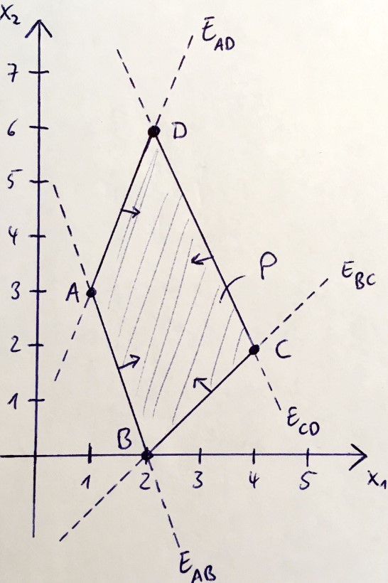
The convex hull is described by all points that lie in the polygon formed between the corners.

We can create the following system of linear equalities:

$$ \begin{aligned} AB: 3x_1 + x_2 = 6 \\ BC: -x_1 + x_2 = -2 \\ CD: -2x_1 - x_2 = -10 \\ AD: 3x_1 - x_2 = 0 \end{aligned} $$

With this, we can create our half-spaces to describe the polyhedron:

$$ A = \begin{pmatrix} 3 & 1 \\ -1 & 1 \\ -2 & -1 \\ 3 & -1 \end{pmatrix}, \quad b = \begin{pmatrix} 6 \\ -2 \\ -10 \\ 0 \end{pmatrix} $$

Thus, we have a polyhedron.

Solution b)

If \(K\) is a finite generated cone, then there exists a matrix \(U\) such that \( K = \{ U \lambda : \lambda \geq 0 \} \), which means the set of all points is a linear combination of the columns in \(U\) that are non-negative.

Let \( I = [-\frac{\pi}{4}, \frac{\pi}{2}] \). We can then write:

$$ \begin{aligned} K &= \{ r (\cos(\phi), \sin(\phi)) : r \geq 0, \phi \in I \} \\ &= \{ r (-\cos(\phi), -\sin(\phi)) : r \geq 0, \phi \in I \} \\ &= \{ U \lambda : \lambda \geq 0 \} \end{aligned} $$

With

$$ U = \begin{pmatrix} -\cos(\frac{\pi}{2}) & -\cos(-\frac{\pi}{4}) \\ -\sin(\frac{\pi}{2}) & -\sin(-\frac{\pi}{4}) \end{pmatrix} $$

6.4.2 Convex Functions

Task:
a) Show that the following functions are convex:
(i) \( f_1(x) = \|x\| \)
(ii) \( f_2(x) = \max\{x_1, \dots, x_n\} \)
(iii) \( f_3(x) = \frac{x_2^2}{x_1} \)
(iv) \( f_4(x) = \exp(a^T x) \)

b) Which of these functions are strictly convex?

Solution a)

(i) \( f_1(\lambda x + (1 - \lambda) y) = \| \lambda x + (1 - \lambda) y \| \leq \lambda \| x \| + (1 - \lambda) \| y \| \), where the last step uses the triangle inequality.

(ii) \( f_2(\lambda x + (1 - \lambda) y) = \max\{\lambda x_1 + (1 - \lambda) y_1, \dots, \lambda x_n + (1 - \lambda) y_n\} \leq \max\{\lambda x_1, \dots, \lambda x_n\} + \max\{(1 - \lambda) y_1, \dots, (1 - \lambda) y_n\} = \lambda f_2(x) + (1 - \lambda) f_2(y) \)

(iii) The gradient and Hessian matrix are:

$$ \nabla f_3(x) = \left( \frac{-x_2^2}{x_1^2}, \ \frac{2 x_2}{x_1} \right), \quad H_f(x) = \begin{pmatrix} \frac{2x_2^2}{x_1^3} & \frac{-2x_2}{x_1^2} \\ \frac{-2x_2}{x_1^2} & \frac{2}{x_1} \end{pmatrix} $$

Using the Hessian, we can show convexity:

$$ \begin{aligned} z^T H_f(x) z &= z_1 \left( \frac{2x_2^2}{x_1^3} z_1 - \frac{2x_2}{x_1^2} z_2 \right) + z_2 \left( \frac{-2x_2}{x_1^2} z_1 + \frac{2}{x_1} z_2 \right) \\ &= \frac{2}{x_1} \left( \frac{x_2}{x_1} z_1 - z_2 \right)^2 \geq 0 \end{aligned} $$

Thus, \( H_f(x) \) is positive definite, and the function is convex.

(iv) Since \( \exp(x) \) is convex, we have:

$$ f_4(\lambda x + (1 - \lambda) y) = \exp(a^T(\lambda x + (1 - \lambda) y)) = \exp(a^T \lambda x + a^T(1 - \lambda) y) \\ \leq \lambda \exp(a^T x) + (1 - \lambda) \exp(a^T y) = \lambda f_4(x) + (1 - \lambda) f_4(y) $$

Thus, \( f_4(x) \) is convex.

Solution b)

(i) Norms are never strictly convex. For example, if \( x \neq 0 \) and \( y = 0 \), then \( \|x\| = \|y\| \), which implies they are equivalent and not strictly greater.

(ii) Not strictly convex. For example, \( \max\{1, 0\} = \max\{1, 0.5\} = \max\{1, 1\} = 1 \), so we can have points with the same function value, which violates the condition for strict convexity.

(iii) Not strictly convex. For example, \( f_3(x_1, 0) = 0 \) for all \( x_1 \), as shown in (ii).

(iv) Not strictly convex for \( a = 0 \).

6.4.3 Duality for Convex Problems

Task:
Given the convex optimization problem

$$ (P) \quad \min \ \ x_1^2 + x_2, \ \ M = \{x \in \mathbb{R}^2 : \| x \|_2 \leq 1\} $$

formulate the dual problem (D) and solve both.

Solution

First, we will check that (P) is indeed a convex problem.

$$ f(x) = x_1^2 + x_2 = x^T Q x + c^T x $$

with

$$ Q = \begin{pmatrix} 1 & 0 \\ 0 & 0 \end{pmatrix}, \quad c = \begin{pmatrix} 0 \\ 1 \end{pmatrix} $$

Since we can write the problem in this form, it is convex.

Next, we can formulate the Lagrange function for the problem.

$$ L(x, u) = f(x) + u^T g(x) + v^T (Ax - b) $$$$ = x_1^2 + x_2 + u (x_1^2 + x_2^2 - 1) = (1 + u)x_1^2 + (u x_2 + 1)x_2 - u $$

From this, we obtain:

$$ F(u) = \inf L(x,u) = \inf_{x_1} \left( (1 + u)x_1^2 \right) + \inf_{x_2} \left( (u x_2 + 1)x_2 \right) - u $$

which has the property \( F(0) = -\infty \). We take the derivative of \( L \):

$$ \nabla_x L(x, u) = \begin{pmatrix} 2(1 + u)x_1 \\ 2ux_2 + 1 \end{pmatrix} $$

Setting \( \nabla_x L(x, u) = 0 \):

$$ \begin{pmatrix} x_1 \\ x_2 \end{pmatrix} \ = \ \begin{pmatrix} 0 \\ -\frac{1}{2u} \end{pmatrix} $$

The minimum is thus:

$$ F(u) = \begin{cases} -\frac{1}{4u} - u, & u > 0 \\ -\infty, & u = 0 \end{cases} $$

We now solve:

$$ \max_u F(u) $$

Analysis shows that \( u^* = \frac{1}{2} \) is the solution from (D) with \( \max(D) = -1 \). By the weak duality lemma, any \( x^* \) such that \( f(x^*) = -1 \) is a solution of (P). For example, the point \( x^* = (0, 1) \in M \).

6.4.4 Duality and Slater Condition

Task:
The function \( g \) is given by

$$ g(x) = \begin{cases} e^x - 2, \quad x < 0, \\ 2x - 1, \quad x \geq 0 \end{cases} $$

And the optimization problem is

$$ \min \ f(x) = -x \quad \text{subject to} \quad g(x) \leq 0. $$

a) Show that \( f \) and \( g \) are convex, and that (P) is a convex optimization problem.
b) Is the Slater condition fulfilled?
c) What is the dual problem (D) to (P)?
d) Solve (P) and (D).
e) Is there a duality gap?

Solution a)

The function \( f \) is linear, and thus convex.

We calculate the first derivatives of \( g(x) \):

$$ g'(x) = \begin{cases} e^x, \quad x < 0 \\ 2, \quad x \geq 0 \end{cases} $$

We check the convexity condition for \( x, y \in \mathbb{R} \) and assume \( x \leq y \):

$$ [g'(y) - g'(x)](y - x) \geq 0. $$

We can then do a case distinction:

(i) \( x, y \in (-\infty, 0): \quad g'(y) - g'(x) = e^y - e^x \geq 0 \)
(ii) \( x \in (-\infty, 0), y \in [0, \infty): \quad g'(y) - g'(x) = 2 - e^x \geq 0 \)
(iii) \( x, y \in [0, \infty): \quad g'(y) - g'(x) = 2 - 2 \geq 0 \)

Thus, the function \( g(x) \) is convex.

Solution b)

The Slater condition is:

(i) \( Rg(A) = m \leq n \)
(ii) There exists \( x' \in \mathbb{R}^n \) such that \( A x' = b \) and \( g_i(x') < 0 \).

We do not have any condition of the form \( A x = b \), so we only need to check the second condition.

We can use any \( x \leq 1/2 \) such that \( g(x) \leq 0 \).

Solution c)

We establish the Lagrange function with \( u \geq 0 \):

$$ L(u) = \inf \left[ f(x) + u^T g(x) \right] = \inf \left[ -x + u^T g(x) \right]. $$

Case 1: \( u = 0 \)

\[ L(0) = \inf[-x] = -\infty. \]

Case 2: \( u > 0 \), then we differentiate:

(i) \( x < 0 \)

$$ L_-(u) = \inf[-x + u(e^x - 2)] = -2u + \inf[-x + ue^x]. $$

For \( 0 < u \leq 1 \),

$$ L_-(u) = -2u - u e^0 = -u. $$

For \( u > 1 \), the function \( -x + ue^x \) is monotonically decreasing on \( (-\infty, -\ln(u)] \) and increasing on \( [-\ln(u), 0) \). Thus,

$$ L_-(u) = -2u + \ln(u) + ue^{-\ln(u)} = -2u + \ln(u) + 1. $$

(ii) \( x \geq 0 \)

$$ L_+(u) = -u + \inf[(2u - 1)x] = \begin{cases} -u, \quad 2u - 1 \geq 0 \\ -\infty, \quad 2u - 1 > 0 \end{cases} $$

Thus, we can bring all cases together:

$$ L(u) = \min \{ L_-(u), L_+(u) \} = \begin{cases} -\infty, \quad u = 0 \\ -\infty, \quad 0 < u < 1/2 \\ -u, \quad 1/2 \leq u \leq 1 \\ -2u + 1 + \ln(u), \quad u > 1 \end{cases} $$

Our dual problem with \( u \geq 1/2 \) is then:

$$ (D) \quad \max \ L(u) = \begin{cases} -u, \quad 1/2 \leq u \leq 1 \\ -2u + 1 + \ln(u), \quad u > 1 \end{cases} $$

Solution d)

The primal problem is feasible because \( g(x) \leq 0 \) if \( x \leq 1/2 \). Further, \( f(x) = -x \geq -1/2 = f(1/2) \) for all \( x \leq 1/2 \).
Thus, the solution is:

$$ \min f(x) = -1/2. $$

The function \( L(u) \) is the dual problem:

$$ \max \ L(u) = L(1/2) = -1/2. $$

Solution e)

There is no duality gap because \( \min(P) = \max(D) \).

6.4.5 Duality and Saddle Point Lemma

Task:
Given:

$$ \min \ \ f(x) = e^{x_1^2 + (x_2 - 1)^2} $$

subject to:

$$ M = \{|x_2| - x_1 \leq 0, \ x_2^2 + x_1 \leq 1\} $$

a) Show that (P) is a convex problem.
b) Show that (P) has a solution.
c) Calculate the solution of (P) using duality and the saddle point lemma.

Solution a)

Let \( h_1 = |x_2| - x_1 \) and \( h_2 = x_2^2 + x_1 - 1 \), with \( \lambda \in [0,1] \):

$$ \begin{aligned} h_1(\lambda x + (1 - \lambda)y) &= |\lambda x_2 + (1 - \lambda)y_2| - (\lambda x_1 + (1 - \lambda)y_1) \\ &\leq \lambda (|x_2| - x_1) + (1 - \lambda)(|y_2| - y_1) \\ &= \lambda h_1(x) + (1 - \lambda) h_1(y) \end{aligned} $$

This shows that \( h_1 \) is convex. To show that \( h_2 \) is convex, we compute:

$$ \nabla h_2(x) = \begin{pmatrix} 1 \\ 2x_2 \end{pmatrix} , \quad \nabla^2 h_2(x) = \begin{pmatrix} 0 & 0 \\ 0 & 2 \end{pmatrix} $$

Since the Hessian matrix is semi-positive definite, \( h_2 \) is convex. Furthermore, both \( h_1 \) and the exponential function \( e^x \) are convex, and the composition of convex functions is convex. Hence, \( f(x) = e^{x_1^2 + (x_2 - 1)^2} \) is convex.

Solution b)

The function \( f(x) \) is a composition of continuous functions, which are smooth and bounded. Furthermore, the set \( M \) is closed and bounded, which makes it compact. According to the Weierstrass Extreme Value Theorem, a continuous function on a compact set always attains a minimum, ensuring that (P) has a solution.

Solution c)

First, let’s consider \( x = (1/2, 0) \in M \). For this point, \( h_1(x) = -1/2 < 0 \) and \( h_2(x) = -1/2 < 0 \), which means this point satisfies the Slater condition and is feasible.

By the strong duality lemma, a solution to the dual problem exists. We define the Lagrangian:

$$ (D) \quad F(u) = \inf \left( e^{x_1^2 + (x_2 - 1)^2} + u_1 (|x_2| - x_1) + u_2 (x_2^2 + x_1 - 1) \right). $$

For a pair \( (x', u') \), the complementary slackness condition \( u'^T h(x') = 0 \) holds. Combining this with the saddle point lemma, we have:

$$ \begin{aligned} & e^{x_1'^2 + (x_2' - 1)^2} + u_1 (|x_2'| - x_1') + u_2 (x_2'^2 + x_1' - 1) \\ & \leq e^{x_1'^2 + (x_2' - 1)^2} + u_1' (|x_2'| - x_1') + u_2' (x_2'^2 + x_1' - 1) \\ & = e^{x_1'^2 + (x_2' - 1)^2}. \end{aligned} $$

We analyze three cases:

1. Case 1: \( u_1' = 0 \):
   With \( x_1 = 0 \) and \( x_2 = 1 \), we get a contradiction.

2. Case 2: \( |x_2'| = x_1' \) and \( u_2' = 0 \):
   This gives a candidate solution \( x' = (1/2, 1/2) \), with \( f(x') = e^{1/2} \).

3. Case 3: \( |x_2'| = x_1' \) and \( x_2'^2 + x_1' - 1 = 0 \):
   This gives \( x' = (1/2, 1/2) \).

Thus, the solution to the problem is \( x' = (1/2, 1/2) \).

7. The Quadratic Problem

In this chapter, we take a look at the quadratic optimization problem:

$$ (P) \quad \text{Minimize} \ \ f(x) := x^T Q x + c^T x \ \ \text{on} \ \ M = \{x \in \mathbb{R}^n : x \geq 0, A x = b\} $$

Where \(Q\) is any quadratic matrix.

Interlude

a) Because \(x^T Q x = x^T Q^T x\), we have:

$$ f(x) = x^T Q x + c^T x = \frac{1}{2} x^T (Q + Q^T) x + c^T x = x^T Q_{\text{Sym}} x + c^T x $$

with \(Q_{\text{Sym}} = \frac{1}{2} (Q + Q^T)\), which is symmetric. This means we can transform any quadratic matrix into a symmetric matrix.

b) If \(Q\) is symmetric and positive definite, then the objective function is convex.

7.1 Existence Lemma and Kuhn-Tucker

Lemma
Let (P) be feasible and \(\inf(P) > - \infty\). Then (P) has a solution.

The lemma from Kuhn-Tucker for quadratic problems is part of the strong duality lemma for linear and convex problems and is also called the Lagrange multiplier lemma.

Lemma (Lagrange Multiplier)
Let \(x^* \in M\) be a solution of the linear problem:

$$ (LP) \quad \text{Minimize} \ \ c^T x \ \ \text{on} \ \ M = \{x \in \mathbb{R}^n : A x = b, x \geq 0\} $$

Then there exists a Lagrange multiplier, i.e., \(y^* \in \mathbb{R}^m\) such that \(c + A^T y^* \geq 0\) and with the equality \((c + A^T y^*)^T x^* = 0\).

For convex problems, we have learned about the Slater condition that needs to be fulfilled for the problem to have a solution. For quadratic problems, we have easier conditions:

Lemma (Kuhn-Tucker)
Let (LP) be the given quadratic optimization problem.

a) Let \(x^*\) be a solution of (P). Then there exists \(y^* \in \mathbb{R}^m\) such that:
(i) \(2 Q x^* + c + A^T y^* \geq 0\) and
(ii) \((2 Q x^* + c + A^T y^*)^T x^* = 0\).

b) Let \(Q\) be symmetric and positive definite, \(x^* \in M\), and there exists \(y^* \in \mathbb{R}^m\) with (i) and (ii). Then \(x^*\) is a solution of (LP).

This lemma can also be formulated for the following canonical form:

$$ (LP2) \quad \text{Minimize} \ \ c^T x \ \ \text{on} \ \ M = \{x \in \mathbb{R}^n : A x \leq b\} $$

Lemma (Kuhn-Tucker)
Let (LP2) be the given quadratic optimization problem.

a) Let \(x^*\) be a solution of (P). Then there exists \(y^* \in \mathbb{R}^m\) such that:
(i) \(2 Q x^* + c + A^T y^* = 0\) and
(ii) \((2 Q x^* + c + A^T y^*)^T x^* = 0\).

b) Let \(Q\) be symmetric and positive definite, \(x^* \in M\), and there exists \(y^* \in \mathbb{R}^m\) with \(y^* \geq 0\), (i), and (ii). Then \(x^*\) is a solution of (LP2).

7.2 Set of Problems and Solutions

7.2.1 Duality and Quadratic Problems

Task: Given a symmetric, positive definite matrix \(Q\), a matrix \(A\), and a vector \(c\), consider the following two quadratic optimization problems:

$$ \begin{aligned} (P1) \quad \min \ \ \frac{1}{2} x^T Q x + c^T x \ \ \text{on} \ \ M = \{A x \leq b\} \\ (P2) \quad \min \ \ \frac{1}{2} y^T A Q^{-1} A^T y + (b + A Q^{-1} c)^T y \ \ \text{on} \ \ M^* = \{y \geq 0\} \end{aligned} $$

Show that:
a) (P1) is unambiguously solvable by an \(x^* \in M\), if \(M\) is not empty.
b) The problem (P2) is equivalent to the dual problem of (P1).

Solution a)

We define \(f(x) = \frac{1}{2} x^T Q x + c^T x\).

The matrix \(Q\) is symmetric and positive definite, thus the second derivative \(D^2 f(x) = Q\), and the function is strictly convex.

If the conditions are fulfilled:

• \(M\) is not empty,
• \(M\) is closed,
• \(f\) is strictly convex,
• \(M\) is convex (since \(A x \leq b\) is the intersection of half-spaces, which is convex),

then (P1) is solvable using the lemma in section 6.2.

Solution b)

To show that (P2) is equivalent to the dual problem of (P1), we investigate the dual problem of (P1).

Let \(g(x) := A x - b\), so that:

$$ M = \{x \in \mathbb{R}^n : g(x) \leq 0\} $$

where \(g\) is a convex function. The dual problem has the form:

$$ (D1) \quad \max \ F(u) \ \ \text{on} \ \ N = \{u \in \mathbb{R}^m : u \geq 0, \ F(u) > -\infty\} $$

with:

$$ F(u) = \inf \left( \frac{1}{2} x^T Q x + c^T x + u^T (A x - b) \right) $$

We consider the necessary condition:

$$ \nabla_x L(x, u) = Q x + c + A^T u = 0 $$

From which we get \(x = -Q^{-1}(c + A^T u)\), and since \(D^2 f(x) = Q\) is symmetric and positive definite, we have a local minimum (which is also a global minimum, since the Lagrange function is convex).

Substituting this into our function:

$$ \begin{aligned} F(u) &= L(-Q^{-1}(c + A^T u)) \\ &= \frac{1}{2} (c + A^T u)^T Q^{-T} Q Q^{-1} (c + A^T u) - c^T Q^{-1} (c + A^T u) - u^T A Q^{-1} (c + A^T u) - u^T b \\ &= \frac{1}{2} (c + A^T u) Q^{-1} (c + A^T u) - (c + A^T u)^T Q^{-1} (c + A^T u) - u^T b \\ &= - \frac{1}{2} (c + A^T u)^T Q^{-1} (c + A^T u) - u^T b \\ &= -\frac{1}{2} u^T A Q^{-1} A^T u - u^T A Q^{-1} c - \frac{1}{2} c^T Q^{-1} c - u^T b \\ &= -\frac{1}{2} u^T A Q^{-1} A^T u - u^T (b + A Q^{-1} c) - \frac{1}{2} c^T Q^{-1} c \end{aligned} $$

Thus, the dual problem is:

$$ \max \ \ -\frac{1}{2} u^T A Q^{-1} A^T u - u^T (b + A Q^{-1} c) - \frac{1}{2} c^T Q^{-1} c $$

This can be transformed into:

$$ \min \ \ \frac{1}{2} u^T A Q^{-1} A^T u + u^T (b + A Q^{-1} c) - \left( - \frac{1}{2} c^T Q^{-1} c \right) $$

Which is the same as (P2) if we set \(y = u\).

8. Differentiable Problems

In this final section, we want to consider one last class of optimization problems, “differentiable problems.” They have the form:

$$ (P) \quad \min f(x), \ \ x \in M = \{x \in \mathbb{R}^n : g(x) \leq 0, h(x) = 0\} $$

with

$$ \begin{aligned} f: \mathbb{R}^n \to \mathbb{R} \\ g: \mathbb{R}^n \to \mathbb{R}^p \\ h: \mathbb{R}^n \to \mathbb{R}^m \\ \end{aligned} $$

all continuously differentiable.

This class of optimization problems also has a Lagrange multiplier rule, just like the other classes. To use this, we need three steps for a local solution \(x^* \in M\):

1. We linearize (P) around \(x^*\), resulting in a linear optimization problem (LP), as seen in the first few chapters.
2. We show that 0 is a solution to the (LP).
3. We use the Kuhn-Tucker lemma on the solution 0.

8.1 Lemma of Lyusternik

Review: Differentiable

We remember that \(g: \mathbb{R}^n \to \mathbb{R}^p\) is differentiable at \(x \in \mathbb{R}^n\) if a matrix \(g'(x) \in \mathbb{R}^{p \times n}\) exists such that

$$ \lim_{h \to 0} \frac{|g(x+h)-g(x)-g'(x)h|}{|h|} = 0 $$

We write this as

$$ g(x + h) = g(x) + g'(x)h + o(|h|), \quad h \to 0 $$

Such a representation also exists for matrices; we call them functional matrices, and they consist of the partial derivatives, for example:

$$ g'(x) = \left( \frac{\partial g_i(x)}{\partial x_j} \right) $$

We can now linearize our problem (P) around our solution \(x^*\). For this, we replace \(f(x)\) with \(f(x^*) + f'(x^*)z\), and so on. We get:

$$ \min f'(x^*)z, \ \ z \in \mathbb{R}^n, \quad g(x^*) + g'(x^*)z \leq 0, \ \ h'(x^*)z = 0 $$

To show that 0 is a solution of the (LP), if \(x^*\) is a solution of (P), we need one more lemma.

Theorem (Implicit Functions)
Let \( H: \mathbb{R}^m \times \mathbb{R} \to \mathbb{R} \) be continuously differentiable. Suppose \( (y', t') \in \mathbb{R}^m \times \mathbb{R} \) with \( H(y', t') = 0 \) and \( \frac{\partial H}{\partial y}(y', t') \in \mathbb{R}^{m \times m} \) is regular (invertible).

\[ \begin{aligned} \implies \exists \, \delta > 0 , \gamma: (t' - \delta, t' + \delta) \to \mathbb{R}^m \text{ such that } \\ \gamma(t') = y' \text{ and } H(\gamma(t), t) = 0 \text{ for all } |t - t'| < \delta. \end{aligned} \]

with \(\gamma\) being continuously differentiable.

The derivative of \( \gamma \) at \( t' \) is obtained using the chain rule:

\[ 0 = \frac{\partial H}{\partial y}(y', t') \gamma'(t') + \frac{\partial H}{\partial t}(y', t') \]\[ \implies \gamma'(t') = - \left( \frac{\partial H}{\partial y}(y', t') \right)^{-1} \frac{\partial H}{\partial t}(y', t') \]

This can be used to prove the following theorem.

Theorem (Lyusternik)
Let \( h: \mathbb{R}^n \to \mathbb{R}^m \) be continuously differentiable with \( h(x^*) = 0 \).
Further, let \( h'(x^*) \in \mathbb{R}^{m \times n} \) have rank \( m \) (i.e., \( m \leq n \)).
Suppose also that \( z \in \mathbb{R}^n \) satisfies \( h'(x^*)z = 0 \).

Then, there exists \( \delta > 0 \) and a continuously differentiable function \( r: (-\delta, \delta) \to \mathbb{R}^n \) such that \( r(0) = 0 \), \( r'(0) = \lim_{t \to 0} \frac{r(t)}{t} \), and \( h(x^* + tz + r(t)) = 0 \) for all \( t \in (-\delta, \delta) \).

8.2 Lagrange Multiplication Rule

We define the Lagrange function for our problem (P):

$$ L : \mathbb{R}^n \times \mathbb{R}^p \times \mathbb{R}^m \to \mathbb{R}, \ \ L(x, u, v) = f(x) + u^Tg(x) + v^T h(x) $$

Definition
Let \((P)\) be given.

i) The conditions \( \Delta L(x,u,v) = 0, \ h(x) = 0, \ g(x) \leq 0, \ u \geq 0, \ u^T g(x) = 0 \) are called Karush-Kuhn-Tucker (KKT) conditions, where \( \Delta L(x,u,v) = \Delta f(x) + u^T g'(x) + v^T h'(x) \).

ii) Any triplet \( (x^*, u^*, v^*) \) that satisfies the KKT conditions is called a KKT point of \((P)\). The components \( (u^*, v^*) \) are called the Lagrange multipliers.

The Slater condition we had for convex problems is replaced here by the constraint qualification (CQ1) condition at \( x \in \mathbb{R}^n \).

i) The rank of \( h'(x) = m < n \).

ii) There exists \( z' \in \mathbb{R}^n \) such that \( g(x) + g'(x) z' < 0 \), and \( h'(x) z' = 0 \).

Remarks

For feasible \( x \in M \), condition ii) can be replaced by:
ii) There exists \( z' \in \mathbb{R}^n \) such that \( g_i'(x) z' < 0 \) for \( i \in I(x) \) (active indices), and \( h'(x) z' = 0 \).

CQ1 is also called the Mangasarian-Fromovitz CQ.

Theorem (Lagrange Rule)
Let \( K \subset \mathbb{R}^n \) be open, and let \( f: K \to \mathbb{R} \), \( g: K \to \mathbb{R}^p \), \( h: K \to \mathbb{R}^m \) be continuously differentiable.
Suppose \( x^* \) is a local minimum of \( f \) on the set

\[ M = \{ x \in K : g(x) \leq 0, h(x) = 0 \}. \]

If (CQ1) holds at \( x^* \), then there exist \( u^* \in \mathbb{R}^p \) and \( v^* \in \mathbb{R}^m \) such that \( (x^*, u^*, v^*) \) is a KKT point of \((P)\).

With this, we know that our KKT points are possible solutions for our optimization problem.

8.3 Necessary and Sufficient Conditions

In this section, we want to look at additional conditions that can be used to determine whether a problem is solvable and to solve it.

We consider the same problem as in the last section:

\[ \min f(x), \quad x \in M = \{ y \in \mathbb{R}^n : g(y) \leq 0, h(y) = 0 \}. \]

Let \( x \in M \), and let \( I(x) = \{ i \in \{ 1, \dots, p \} : g_i(x) = 0 \} \) denote the active indices.

The vectors:

\[ \{ g_i'(x) : i \in I(x) \} \cup \{ h_j'(x) : j \in \{ 1, \dots, m \} \} \]

are linearly independent.

Thus, if \( I = T(x^*) = \{ i_1, \dots, i_q \} \) with \( 1 \leq i_1 \leq \dots \leq i_q \) and \( g_I(x) = (g_{i_j}(x)) \), then (CQ2) means exactly that:

\[ \text{Rank} \left( \begin{pmatrix} g'_I \\ h'(x^*) \end{pmatrix} \right) = q + m \]

Lemma
If (CQ2) is optimal, then (CQ1) also holds. So, \( \text{CQ2} \implies \text{CQ1} \).

Theorem
Let \( x^* \) be a local minimum of \( f \) on \( M \) and suppose (CQ2) holds. Additionally, let \( f \), \( g \), and \( h \) be twice continuously differentiable at \( x^* \). Then there exist \( u^*, v^* \) with \( u^* \geq 0 \) such that:

• a) \( L(x^*, u^*, v^*) = 0 \), i.e., we have a KKT tuple.
• b) \( u_i^* g_i(x^*) = 0 \).
• c) Define the subspace

\[ V = \{ z \in \mathbb{R}^n : h'(z) = 0, g_i(x^*)^T z = 0 \}. \]

Then

\[ z^T L z \geq 0 \]

which means it is positive semi-definite on \( V \).

Theorem
Let \( (x^*, u^*, v^*) \) be a KKT point of \( (P) \), and let \( I^* = I(x^*, u^*) = \{ i \in I(x^*) : u_i^* > 0 \} \) denote the strongly active indices. Assume that \( f \), \( g \), and \( h \) are \( z \)-times continuously differentiable.
Furthermore, suppose that \( L(x^*, u^*, v^*) \) is positive definite on the cone:

\[ K = \{ z \in \mathbb{R}^n : h'(x^*) z = 0, g'(x^*) z = 0, g_i'(x^*) z < 0, i \in I \setminus I^+ \}. \]

Then

\[ z^T L(x^*, u^*, v^*) z > 0 \quad \forall z \in K \]

This implies that \( x^* \) is a strict local minimum.

8.4 Further Optimality Criteria

In this section, we discuss a constraint qualification that is weaker than \((CQ1)\).

Definition
Let \( \emptyset \neq X \subset \mathbb{R}^n \). A vector \( d \in \mathbb{R}^n \) is called tangential to \( X \) at a point \( x \in X \) if there exists a sequence \( \{x^k\} \subset X \) and \( \{t_k\} \subset (0, \infty) \) such that

\[ x^k \to x, \quad t_k \to 0, \quad \frac{x^k - x}{t_k} \to d. \]

The set of all such directions is called the tangent cone of \( X \) at \( x \in X \), denoted \( T_X(x) \).

Example

If the set \( X \) is a rectangle and the point \( x \) lies somewhere in the middle, then \( T_x(X) = \mathbb{R}^2 \). If the point \( y \) is at the upper-right corner, then \( T_y(X) = \{d \in \mathbb{R}^2 : d_1 \leq 0, d_2 \leq 0 \} \)

Lemma
Let \( \emptyset \neq X \subset \mathbb{R}^n \), and let \( x \in X \). Then \( T_x(X) \) is closed.

Lemma
Let \( \emptyset \neq X \subset \mathbb{R}^n \), \( f: \mathbb{R}^n \to \mathbb{R} \) be continuously differentiable, and let \( x^* \in X \) be a local minimum of \( f \) over \( X \). Then the following holds:

\[ f'(x^*) d \geq 0 \quad \forall d \in T_X(x^*) \]

The critical or stationary points of a constrained optimization problem are therefore all \( x^* \in X \) such that

\[ \Delta f(x^*) d \geq 0 \quad \forall d \in T_X(x^*) \]

Only these points are candidate Lagrange multiplier points. For \( T_X(x^*) = \mathbb{R}^n \), we get the usual condition \( \Delta f(x^*) = 0 \).

We now consider the following problem:

\[ \min f(x), \quad x \in M = \{ z \in \mathbb{R}^n : g(z) \leq 0, h(z) = 0 \} \]

Definition
Let \( x \in M \). The linearized tangent cone of \( M \) at \( x \) is defined as

\[ T_{\text{lin}}(x) = \{ d \in \mathbb{R}^n : g_i'(x) d \leq 0, \, i \in I(x), \, h'(x) d = 0 \}, \]

where \( I(x) \) is the set of active indices.

Lemma
Let \( x \in M \). Then \( T_M(x) \subset T_{\text{lin}}(x) \).

If

\[ T_M(x) = T_{\text{lin}}(x), \]

we refer to this as ACQ (Active Constraint Qualification).

Theorem (Multiplier Rule under ACQ)
Let \( f \), \( g \), and \( h \) be differentiable, and let \( x^* \) be a local minimum of \( f \) in \( M \). Suppose (ACQ) holds at \( x^* \).
Then there exists a KKT point \( (x^*, u^*, v^*) \).

As an application of the previous theorem, consider the linear restricted optimization problem (LRP):

\[ \min f(x), \quad x \in M = \{ \phi \in \mathbb{R}^n : B \phi \leq c, \, A \phi = b \}, \]

where \( f \) is continuously differentiable.

Theorem
Under the above assumption, if \( x^* \in M \) is a local minimum of LRP, then there exists a KKT point \( (x^*, u^*, v^*) \) for LRP, i.e.,

\[ \Delta f(x^*) + (u^*)^T B + (v^*)^T A = 0, \quad u^* \geq 0, \quad B x^* \leq c, \quad A x^* = b, \quad (u^*)^T (B x^* - c) = 0. \]

Theorem
It holds that

\[ \text{CQ1} \implies \text{ACQ}. \]

Quadratic Problems with Linear Constraints

\[ \min f(x) = x^T Q x + c^T x, \quad x \in M = \{ \phi \in \mathbb{R}^n : \phi \geq 0, \, A x = b \} \quad (QP), \]

with \( Q = Q^T \), \( b \in \mathbb{R}^m \).

Theorem
If (QP) is feasible and \( \inf (QP) > -\infty \), then (QP) has a local minimum solution.

Theorem (Multiplier Rule)
a) Let \( x^* \in M \) for (QP) \( \implies \) there exist \( u^*, v^* \) such that

\[ 2Qx^* + u^* + A^T v^* = 0. \]

b) Let \( Q \) be positive semi-definite, and \( x' \in M \) with \( \exists u', v' \) such that

\[ 2Qx' - u' + A^T v' = 0, \quad u'^T x' = 0, \]

then \( x' \) is a local minimum solution of (QP).

This is a very important theorem, which helps us in solving differentiable optimization problems.

Theorem (necessary second-order optimality conditions)
Let \( x^* \) be a local minimum of \( f \) on \( M \), and let (CQ2) hold. Furthermore, assume that \( f, g \), and \( h \) are twice continuously differentiable at \( x^* \). Then there exist \( u^* \in \mathbb{R}^p \), \( v^* \in \mathbb{R}^m \), with \( u^* \geq 0 \), such that:

(a)

\[ \nabla_x L(x^*, u^*, v^*) = 0 \]

where the Lagrangian function is defined as

\[ L(x, u, v) = f(x) + u^\top g(x) + v^\top h(x), \quad x \in \mathbb{R}^n, \, u \in \mathbb{R}^p, \, v \in \mathbb{R}^m. \]

(b)

\[ u_i^* g_i(x^*) = 0 \quad \text{for all } i = 1, \dots, p. \]

(c) Define the subspace

\[ V = \left\{ z \in \mathbb{R}^n : h(x^*)^\top z = 0, \, \nabla g_i(x^*)^\top z = 0 \text{ for all } i \in I(x^*) \right\}. \]

Then it holds that

\[ z^\top \nabla_x^2 L(x^*, u^*, v^*) z \geq 0 \quad \text{for all } z \in V, \]

i.e.,

\[ \nabla_x^2 L(x^*, u^*, v^*) \]

is positive semidefinite on \( V \).

Theorem (Second-Order Sufficient Optimality Condition)
Let \((x^*, u^*, v^*) \in \mathbb{R}^n \times \mathbb{R}^p \times \mathbb{R}^m\) be a Kuhn-Tucker point, meaning that \(x^* \in M\), \(u^* \geq 0\), and \(u_i^* g_i(x^*) = 0\) for all \(i = 1, \dots, p\), as well as

\[ \nabla_x L(x^*, u^*, v^*) = 0. \]

Assume that the functions \( f \), \( g \), and \( h \) are twice continuously differentiable at \( x^* \). Furthermore, suppose the Hessian \( \nabla_x^2 L(x^*, u^*, v^*) \) is strictly positive definite on the cone

\[ K = \{ z \in \mathbb{R}^n : h'(x^*) z = 0, \, \nabla g_i(x^*)^T z = 0 \text{ for } i \in I^+, \, \nabla g_i(x^*)^T z \leq 0 \text{ for } i \in I(x^*) \setminus I^+ \} \]

which means:

\[ z^T \nabla_x^2 L(x^*, u^*, v^*) z > 0 \quad \text{for all } z \in K, \, z \neq 0. \]

Then \( x^* \) is a strict local minimum of \( f \) on \( M \).

8.5 Set of Problems and Solutions

8.5.1 CQ1/Mangasarian-Fromowitz-Condition

Task: Use the Lagrange multiplication rule on the set

$$ M = \{(x,y) \in R^2 \ : \ y^2 = (x+1)(x-1)^2\} $$

to get all points with the minimum distance to the origin.

Solution

The function \(f(x,y) = x^2 + y^2\) and \(g(x,y) = y^2 -(x+1)(x-1)^2\) are differentiable. Thus, we can write the problem as a differentiable problem:

$$ (P) \quad \min \ \ f(x,y) \ \ \text{on} \ \ M = \{(x,y) \in R^2 \ : \ g(x,y) = 0\} $$

A sketch of \(M\):

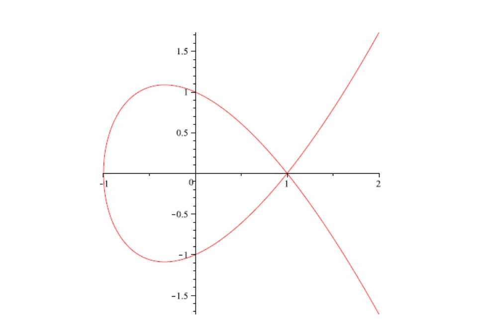
The Lagrange function is given by:

$$ L(x, y, v) = f(x, y) + vg(x,y) = x^2 + y^2 + vy^2 - v(x+1)(x-1)^2 $$

The CQ1 condition is then fulfilled when \(Rg(g'(x,y))\) is maximal.
If we derive \(g\), we obtain a \(1 \times 2\) matrix, meaning the minimum row/column rank is 1, and thus \(\max Rg(g'(x,y)) = 1\).

Thus, for CQ1 to be fulfilled, \(\nabla g(x,y) \neq 0\), meaning:

\[ \begin{aligned} & \frac{\partial g}{\partial y}(x,y) = 2y = 0 \\ & \frac{\partial g}{\partial x}(x,y) = -\left[(x-1)^2 + 2(x+1)(x-1)\right] = -(x-1)(3x+1) = 0 \end{aligned} \]

which is fulfilled for \(x \in \{1, -1/3\}, y=0\). The point \((-1/3, 0)\) is not in \(M\), but the point \((1, 0)\) is in \(M\).

The Lagrange rule does not provide information about the point \((1,0)\), thus we need to check it separately. We calculate \(f(1,0)=1\). In other words, \((-1/3, 0)\) is not a possible solution (because it is not in \(M\)), but \((1,0)\) is a possible solution.

If \((x,y) \neq (1,0)\) is a local minimum of \(f\) on \(M\), then there exists a \(v \in R\) such that \(\nabla L(x,y,v) = 0\), according to the Lagrange rule. Furthermore, since \((x,y) \in M\), we have \(g(x,y) = 0\). From this, we can formulate the following equations by differentiating \(L\) with respect to its three variables:

$$ \begin{aligned} & 2x - v(x-1)(3x +1) = 0 \\ & 2y(1+v) = 0 \\ & y^2 - (x + 1)(x-1)^2 = 0 \end{aligned} $$

From the second equation, it follows that \(y=0\) or \(v =-1\).

Case 1: \(y=0\): From the third equation, we get \(x \in \{-1, 1\}\). The point \((1,0)\) was already considered above. Furthermore, we get \(f(-1, 0) = 1\).

Case 2: \(y \neq 0, v=-1\): From the first equation, we find that \(0 = 3x^2 -1 \), thus \(x_{1,2} = \pm\sqrt{1/3}\). From the third equation, we get the critical points:

\[ P_1 = \begin{pmatrix} -\sqrt{\frac{1}{3}}, -\left(\sqrt{\frac{1}{3}} + 1\right), \sqrt{1 - \sqrt{\frac{1}{3}}} \end{pmatrix}^{\top}, \]\[ P_2 = \begin{pmatrix} -\sqrt{\frac{1}{3}}, \sqrt{\frac{1}{3}} + 1, \sqrt{1 - \sqrt{\frac{1}{3}}} \end{pmatrix}^{\top}, \]\[ P_3 = \begin{pmatrix} \sqrt{\frac{1}{3}}, \sqrt{\frac{1}{3}} - 1, \sqrt{1 + \sqrt{\frac{1}{3}}} \end{pmatrix}^{\top}, \]\[ P_4 = \begin{pmatrix} \sqrt{\frac{1}{3}}, -\left(\sqrt{\frac{1}{3}} - 1\right), \sqrt{1 + \sqrt{\frac{1}{3}}} \end{pmatrix}^{\top}. \]

Thus, we obtain:

$$ \begin{aligned} \min(P) &= \min\{f(-1,0), f(P_1), f(P_2), f(P_3), f(P_4), f(1,0)\} \\ &= \min\{1, 1 + \frac{2}{9}\sqrt{3}, 1- \frac{2}{9}\sqrt{3}\} \\ &= 1- \frac{2}{9} \sqrt{3} \end{aligned} $$

Hence, the points with the smallest distance are \(P_3\) and \(P_4\). Their distance is:

$$ \sqrt{1- \frac{2}{9} \sqrt{3}} $$

8.5.2 Violated CQ1/Mangasarian-Fromowitz Condition

Task: For \(\alpha \in \mathbb{R}\), we have the functions

$$ f(x) = x_1 + x_2 \sin \alpha , \quad h_1(x) = (x_1 - 1)^2 + x_2^2 - 1 , \quad h_2(x) = (x_1 + 1)^2 + x_2^2 -1 $$

Furthermore, we have the optimization problem

$$ (P) \quad \min \ f(x) \ \ \text{subject to} \ \ M = \{x \in \mathbb{R}^2 : h(x) = 0\} $$

where \(h(x) = (h_1(x), h_2(x))\).

a) Draw the level lines for \(h_1, h_2\) and determine the feasible set \(M\), and the solution \(x^*\) for (P).
b) Show that for \(x^*\), CQ1 is not fulfilled.
c) Determine all \(\alpha\) such that a \(v^*\) exists with

$$ \nabla f(x^*) + \sum v_k^* \nabla h_k(x^*) = 0 $$

Solution a)

The feasible set contains only one element: \( M = \{(0,0)\} \). Thus, \( x^* = (0, 0) \) is the solution for (P), with \(\min(P)=0\).

Solution b)

The following holds:

\[ \nabla f(x) = \begin{bmatrix} 1 \\ \sin \alpha \end{bmatrix}, \quad \nabla h_1(x) = \begin{bmatrix} 2x_1 - 2 \\ 2x_2 \end{bmatrix}, \quad \nabla h_2(x) = \begin{bmatrix} 2x_1 + 2 \\ 2x_2 \end{bmatrix} \]

By inserting \(x^*\):

\[ \nabla f(x^*) = \begin{bmatrix} 1 \\ \sin \alpha \end{bmatrix}, \quad \nabla h_1(x^*) = \begin{bmatrix} -2 \\ 0 \end{bmatrix}, \quad \nabla h_2(x^*) = \begin{bmatrix} 2 \\ 0 \end{bmatrix} \]

The vectors \(\nabla h_1(x^*)\) and \(\nabla h_2(x^*)\) are linearly dependent, thus:

\[ \text{rank } h(x^*) = 1 \neq 2 = K \]

Hence, CQ1 is not fullfilled.

Solution c)

Since the CQ1 condition is violated, we cannot directly apply the Lagrange multiplier rule.

We seek a \(v \in \mathbb{R}^2\) such that:

$$ 0 = \nabla_x f(x^*) + v^*{}^T D_x h(x^*) = \begin{bmatrix} 1 \\ \sin \alpha \end{bmatrix} + v_1 \begin{bmatrix} -2 \\ 0 \end{bmatrix} + v_2 \begin{bmatrix} 2 \\ 0 \end{bmatrix} $$

If \(\sin \alpha \neq 0\), then such a \(v\) does not exist.

Now, let \(\sin \alpha = 0\), meaning \(\alpha = n \pi, \quad n \in \mathbb{N}\). In this case, the equation simplifies to \(-1 = -2v_1 + 2v_2\), which implies \(v = (\phi, \phi - 1/2)\) with \(\phi \in \mathbb{R}\) as a Lagrange multiplier.

8.5.3 CQ2/Second-Order Condition

Task: The function \(f(x) = x_1^2 x_2\) with

$$ (P) \quad \min \ f(x) \ \ \text{subject to} \ \ M = \{x \in \mathbb{R}^2 \ : \ ||x||^2 - 4 = 0\} $$

is a differentiable optimization problem.

a) Determine all KKT points of (P).
b) Show, using the necessary second-order optimality condition, that \(f\) has no local minimum at \(x^* = (0,-2)\).
c) Show, using the sufficient second-order optimality condition, that \(f\) has a strict local minimum at \(x^* = (0,2)\).

Solution: Preliminary

We can rewrite the constraint as \(g(x) := x_1^2 + x_2^2 -4 = 0\). Thus, the Lagrangian function is given by:

$$ L(x_1, x_2, v) = x_1^2x_2 + v(x_1^2 + x_2^2 -4 ) $$

Solution a)

The KKT points of (P) are characterized by the conditions \(\nabla_x L(x,v) = 0\) and \(g(x)=0\), which results in the system:

$$ \begin{aligned} 2x_1 (x_2 + v) &= 0 \\ x_1^2 + 2 v x_2 &= 0 \\ x_1^2 + x_2^2 &= 4 \end{aligned} $$

Case 1: \(x_1 = 0\). Then \(x_2 = \pm 2\), and \(v = 0\).

Case 2: \(x_1 \neq 0\). Then \(x_2 = -v\), and with this:

$$ x_1^2 - 2v^2 = 0, \quad x_1^2 + v^2 = 4 $$

By subtracting the equations, we obtain \(3v^2 = 4 \Rightarrow v = \pm \frac{2}{\sqrt{3}}\).
The associated points are:

$$ \left( \pm \frac{2\sqrt{2}}{\sqrt{3}}, -\frac{2}{\sqrt{3}} \right), \quad \left( \pm \frac{2\sqrt{2}}{\sqrt{3}}, \frac{2}{\sqrt{3}} \right) $$

Thus, we have 6 KKT points: 4 from the second case and 2 from the first case.

Solution b)

The constraint qualification (CQ2) is satisfied because:

$$ \nabla g(x) = \begin{pmatrix} 2x_1 \\ 2x_2 \end{pmatrix} \neq \begin{pmatrix} 0 \\ 0 \end{pmatrix} $$

The Hessian matrix of the Lagrangian is:

$$ \nabla^2_x L(x_1, x_2, v) = \begin{pmatrix} 2x_2 + 2v & 2x_1 \\ 2x_1 & 2v \end{pmatrix} $$

If \(f\) had a local minimum at \(x^* = (0, -2)\) with \(v^* = 0\), then the Hessian of the Lagrangian on the subspace

$$ K = \{z \in \mathbb{R}^2 \ : \ g'(x^*)z = 0\} $$

would need to be positive semidefinite. However:

$$ z^T \nabla^2 L(0,-2,0)z = z^T \begin{pmatrix} -4 & 0 \\ 0 & 0 \end{pmatrix} z = -4z_1^2 < 0, \quad \forall z \in K $$

Thus, there is no local minimum at the point \(x^* = (0, -2)\).

Solution c)

Since we only have equality constraints and no inequalities in the set \(M\), we can again examine the cone \(K\) from part (b).

$$ z^T \nabla^2 L(0,2,0)z = z^T \begin{pmatrix} 4 & 0 \\ 0 & 0 \end{pmatrix} z = 4z_1^2 > 0, \quad \forall z \in K $$

Thus, \(f\) has a strict local minimum at the point \(x^* = (0, 2)\).

8.5.4 Minimal Distance to a Point and a Parabola

Task: Find a point \(x \in \mathbb{R}^2\) on the parabola \(4x_2 = x_1^2\) that has the minimum distance to the point \((2,5)\).

Solution

We first need to transform our problem into an optimization problem:

$$ (P) \quad \min \ ||x-(2,5)||^2 \ \ \text{subject to} \ \ P = \{z \in \mathbb{R}^2 \ : \ 4z_2 = z_1^2\} $$

The Lagrangian function is given by:

$$ L(x, v) = (x_1 - 2)^2 + (x_2 - 5)^2 + v(x_1^2 - 4 x_2) $$

Now, we determine the KKT points:

$$ \begin{aligned} &0 =^! \nabla L(x,v) = \begin{pmatrix} 2(x_1 - 2) + 2vx_1 \\ 2(x_2 - 5) - 4v \end{pmatrix} \\ & 0 =^! x_1^2 - 4x_2 \end{aligned} $$

From this, it follows that:

$$ v = \frac{1}{2} x_2 - \frac{5}{2} = \frac{1}{8} x_1^2 - \frac{5}{2} $$

Substituting into the first equation:

$$ 0 = x_1 - 2 + vx_1 = x_1 - 2 + \frac{1}{8}x_1^3 - \frac{5}{2} x_1 $$

This simplifies to:

$$ 0 = x_1^3 - 12 x_1 - 16 = (x_1 + 2)^2 (x_1 - 4) $$

Thus, the solutions are \(x_1 = -2\) or \(x_1 = 4\), leading to the KKT points:

$$ (-2, 1, -2), \quad (4, 4, -1/2) $$

We can now compare their distances:

$$ ||(-2,1) - (2,5)||^2 = 32 > 5 = ||(4,4)-(2,5)||^2 $$

Hence, the point of interest is \((4,4, -1/2)\), for which CQ2 is trivially satisfied.

We now use the sufficient second-order optimality condition:

$$ \nabla^2 L(x^*, v^*) = \begin{pmatrix} 2 + 2v & 0 \\ 0 & 2 \end{pmatrix} = \begin{pmatrix} 1 & 0 \\ 0 & 2 \end{pmatrix} $$

Since the matrix is positive definite, the point \((4,4)\) is a local minimum, and therefore, the point we searched for with the minimal distance to \((2,5)\).

9. Conclusion

This article is by no stretch of the imagination complete, highly accurate, or very intuitive and understandable. It is more like hastily written notes from my lecture combined with various external materials.
The most use one can get from this article is to use it as a reference for theorems or to calculate through the problem solution set, where the solutions should be fairly accurate.

---

Ressources:

• The Lecture “Optimization Theory” by Andreas Kirsch
• The Lecture “Optimization Theory” Martin Frank
• The Book “Einführung in die Mathematische Optimierung” by Rainer Burkard and Uwe Zimmerman
• Princeton Optimization theory