Introduction to Convolutional Neural Network

Published: December 22, 2023

Background

I wrote this article back in uni as part of the seminar, "Basics of Machine Learning 1 & 2". As such this text only introduces some basic concepts and is limited in scope.

Abstract

In recent years, significant advancements have been made in the field of Machine Learning, particularly in the domain of image-related tasks. This paper aims to provide a comprehensive overview of Convolutional Neural Networks (CNNs), a powerful class of neural networks widely employed for image analysis and processing. In addition to that, this paper presents a self-trained CNN model specifically designed for digit classification. The model achieves solid performance in accurately classifying hand-drawn digits. By shedding light on the inner workings of CNNs and showcasing their practical application in digit classification, I seek to encourage further research and development in this domain.

1. Introduction

A study revealed that over 24,000 GB of data is uploaded to the internet every second, from which approximately 80% consists of Video Data [1] . Consequently, a vast amount of visual data is generated each second, highlighting the significance of algorithms capable of comprehending visual information.

Algorithms that can interpret visual data have various applications, including autonomous vehicles that rely on cameras to perceive the environment, analyze it, and make informed decisions based on the gathered data. Additionally, these algorithms are instrumental in fields such as skin cancer detection, robotics, crop disease detection, and more. Therefore, the development of algorithms that possess the ability to understand visual data is rather important.

1.1 Semantic Understanding Of Images: Challenges And A Solution

In computer systems, an image is represented as a matrix, where the size of the matrix corresponds to the dimensions of the image. For instance, if we have an Image with the size of 1920×1080 pixels then the Matrix representation will have the same size, with each entry in the Matrix representing a pixel value in the Image. In the case of a black-and-white image, a single matrix is sufficient to represent the image. However, for colored images, we require separate matrices for each color channel, typically represented by the Red, Green, Blue (RGB) values. Therefore, to represent a colored image, we need a tensor of size 3×1920×1080, so we have three matrices with the size 1920×1080.

This matrix representation poses several challenges for algorithms aiming to understand images, including viewpoint variations, illumination changes, occlusions, background clutter, and more. For Instance, when viewing an image from different perspectives or under different lighting conditions, the semantic meaning remains the same, but the values within the matrix can change drastically.

This brings us to the fundamental question: How can we develop algorithms that can effectively understand images despite the inherent variability in their representations?

One Idea is instead of using rigid rules and handcrafted feature, we let the Computer learn the semantic meaning of Images.

2. Convolutional Neural Network

The paper [2] proved that Neural Network serve as universal function approximator, capable of learning to approximate a given function. This property makes them a suitable candidate for training algorithms to achieve semantic understanding of images. However, as highlighted in this research paper [8], conventional neural networks are not optimally designed for learning visual data due to the following reasons:

A fully connected Neural Network would take too many parameters, thus being computational very expensive to train.
A fully connected Neural Network have no built-in invariance to image transformed like already named in subsection 1.1.
fully connected Neural Networks ignore how the input is ordered, we could randomly map (fixed) input pixels to the first layer without affecting the training.

A more effective approach is to utilize specialized architectures known as convolutional neural networks (CNNs), like introduced in [6], [7] and [8]. These CNNs address the limitations faced by traditional neural networks and provide improved performance in handling visual data.

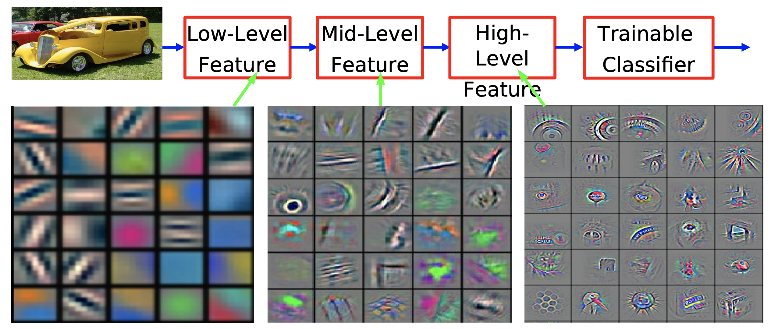
CNNs can learn to semantically understand images, instead of relying on handcrafted features or explicit rules. CNNs do that by learning a hierarchical representation from the raw pixel data, like seen in figure 1.

Figure 1: Feature visualization of convolutional net trained on ImageNet from [10]. Images to the left are features extracted in earlier layers, while images to the right are features extracted in later layer. We can see earlier layer look for more simple patterns while later layer look for more complex pattern. Source: Alfredo Canziani Book Deep Learning.

2.1 Convolutional Neural Network

Convolutional neural networks (CNNs) combine several key ideas:

Local Receptive Fields: Each neuron in the Neural Network receives Input from neighboring neurons in a small local region of the previous layer.
Weights Sharing: Neurons within the same layer share the same set of weights, as opposed to having individual weights for each neuron.
Spatial Subsampling: Subsampling is performed based on region, reducing the dimension of the neural network.

The underlying concept of CNNs is inspired by the functioning of neurons in the visual cortex of animals and humans. This idea dates back to a paper by Hubel and Wiesel [3] in 1960. Where they demonstrated that neurons in the brain of a cat are hierarchically organized and possess local receptive fields. These local receptive fields enable the detection of elementary patterns such as edges, vertices, corners, and more.

To implement this concept, weight sharing is employed. Neurons within the same layer share an identical set of weights, leading to a reduction in the number of parameters in the neural network. This set of weight is also called a filter/kernel. This not only makes training and usage of the network more computationally efficient, but also ensures that the network attends to the same patterns across the entire image. These elementary patterns, identified by the kernel, are also referred to as features and are crucial building blocks for the semantic understanding of the image.

Subsequent layers in the network combine these elementary patterns to form more complex features. A collection of neurons within a layer is commonly referred to as a feature-/activation-map, where all neurons share the same set of weights. This design constraint enables the network to perform the same convolutional operation across different parts of the image.

Within a single convolutional layer, multiple filter/kernel can be employed, each focusing on different features within the image. For instance, we could have one filter which focuses on detecting edges, while another filter identifies corners.

2.2 Convolutional Operation

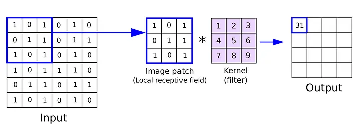
Figure 2: Example of a convolution operation. We have an input matrix, take an input patch out of it, multiply it with the kernel matrix to get the first value of our output. To get the subsequent values, we take the next image patches and do the same process again. Source: Medium @draj0718

The convolutional operation in the 1-dimensional case with the input $x$ and the weight matrix $w$ can be expressed mathematically as follows:

$$ y_{i} = \sum_{j} w_{j} x_{i−j} $$

This is the same as computing the i-th output of a dot product in reverse, in practice we just compute the standard dot product. Thus, the operation can also be understood as a matrix operation, where a weight matrix also known as filter/kernel, is multiplied with a corresponding section of the image matrix. For images as input, we use the two-dimensional formula for convolution:

$$ y_{ij} = \sum_{kl} w_{kl} x_{i+k} $$

Where $y_{ij}$ is an entry in the output matrix. This process is visually illustrated in the figure 2.

The outcome of a single operation is the value assigned to a single neuron in the subsequent layer. By sliding a kernel over the entire image matrix and performing the convolution operation, we obtain the values for the subsequent layer, which are commonly referred to as the feature map.

Two important hyperparameters are associated with the convolution operation:

The first is stride, which determines the number of pixel the kernel slides by during each operation. For example, a stride of 1 means that the sliding window moves 1 pixel at a time.
The second Hyperparameter is the kernel size, which determines the dimensions of the kernel sliding over the input image. For instance, a kernel size of 4×4 indicates that we have a kernel matrix of size 4×4 that slides over the input matrix.

The kernel size can also be understood as the size of the local receptive field of the neurons.

2.3 Subsampling

Training an infinitely large neural network is not feasible due to the increasing computational costs associated with both training and inference. Therefore, it is essential to ensure that a network is not unnecessarily larger than necessary. One way to achieve this is by reducing the dimensions of the network layers, where the dimension means the number of neurons in a layer.

To accomplish dimension reduction, subsampling techniques can be employed. Two popular subsampling methods are average pooling and max pooling.

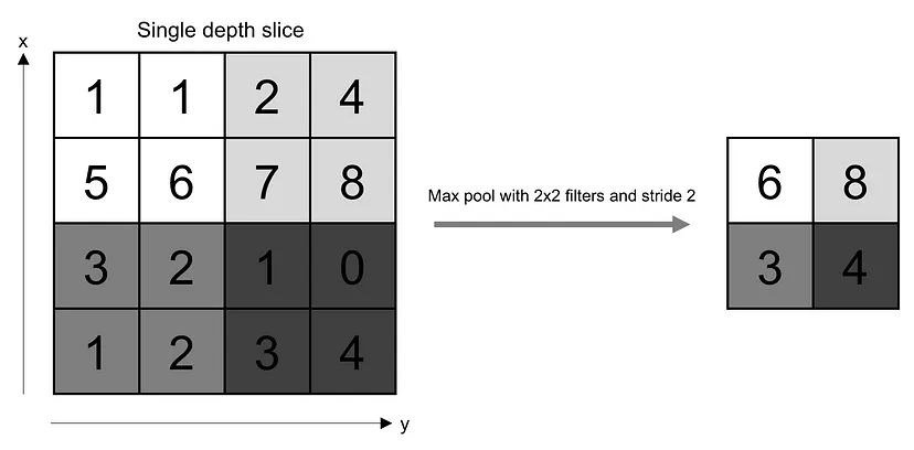
Figure 3: Demonstration of the max-pooling operation with stride 2 and filter size 2x2. We go over each image patch and take the highest value. Source: O’Reilly Media

In average pooling, similar to convolution layers, we slide over our image matrix and take the average of a neighborhood region in the Image and map it to a single neuron in the next layer. On the Figure 3 : Demonstration of the max-pooling operation with stride 2 and filter size 2x2. We go over each image patch and take the highest value. Source: O’Reilly Media other hand, in max pooling, the highest value within a neighborhood region is selected and mapped to a neuron in the subsequent layer. This can be seen as propagating only the most significant signal that excites a neuron while discarding the rest. This approach bears some resemblance to the way the brain processes information. Max pooling is generally more popular than average pooling.

Both of these approached aid in reducing the dimension of the network.

3. Self-Trained CNN

In order to demonstrate the effectiveness of a CNN, I conducted an experiment where I trained a CNN from scratch to recognize black-and-white digits from images.

3.1 Dataset

I trained my CNN using the MNIST dataset [8], the MNIST dataset is a collection of 70,000 hand-drawn digits. These digits have been normalized to fit within a 28×28 pixel bounding box and are gray scaled images. I choose this dataset due to its popularity within the machine learning community and its low computational requirements.

The MNIST dataset is divided into 60,000 training images and 10,000 testing images. By default, the MNIST dataset consists of images with white digits on a black background. However, to enhance the usefulness of the dataset, I inverted the color of all images, making the background white and the digits black.

Figure 4: Sample Data from the MNIST dataset after the preprocessing got applied, but before the color got inverted.

For the alternative models, I applied various additional transformations to the images. Firstly I randomly cropped images, this random cropping helps to augment the dataset, by introducing variation in digit position. Since not all digits are perfectly centered, it will help the model to generalize to different digit locations. Furthermore, I introduced random noise to the image, by sampling from a Bernoulli-Distribution with a probability of 0.7. By doing so, the hope is that the model becomes more robust to noise in the input data. An example of this preprocessing can be seen in figure 4.

3.2 Architecture

Description of the image — Figure 5: The architecture of the Baseline Model. General Matrix multiplication (Gemm) is the same as a fully connected layer.

The CNN architecture, like illustrated in Figure 5, consists of 5 layers with learnable weights. The initial 3 layers are convolutional, while the subsequent 2 layers are fully connected.

The first convolutional layer takes a 28×28×1 image as input and applies 16 filters. The output of the first convolutional layer serves as the input for the second convolutional layer, which further processes it using 64 filters. Lastly, the third convolutional layer employs 16 filters. All convolutional layers employ a kernel size of 4 and a stride of 1.

Following the convolutional layers, the fully connected layers contain 5776, 200, and 10 neurons, respectively. As activation function, Leaky ReLU is applied to all layers except the last one.

The final layer’s output is passed through a 10-way softmax function, generating a probability distribution across 10 class labels. Each neuron in this layer corresponds to a specific digit label, where neuron 0 represents digit 0, neuron 1 represents digit 1, and so on.

3.3 Trainings-Details

The model was trained using the backpropagation algorithm and the cross entropy loss function, which is commonly used for multi-class classification tasks.

For efficient training, Google Colab was used, taking advantage of the free dedicated GPU to accelerate the training process.

The CNN was trained for 5 epochs using a batch size of 1024. The total training time was approximately 5 minutes.

As trainings optimizer, Adam was used with a learning rate of 0.001. Adam is a state-of-the-art optimizer known for its ability to adaptively adjust learning rates during training and the use of momentum [5]. The activation function used in the CNN was Leaky-ReLU, initialized with a slope of 0.2, this value was determined to be effective based on findings from the paper [9].

3.4 Results & Ablation Study

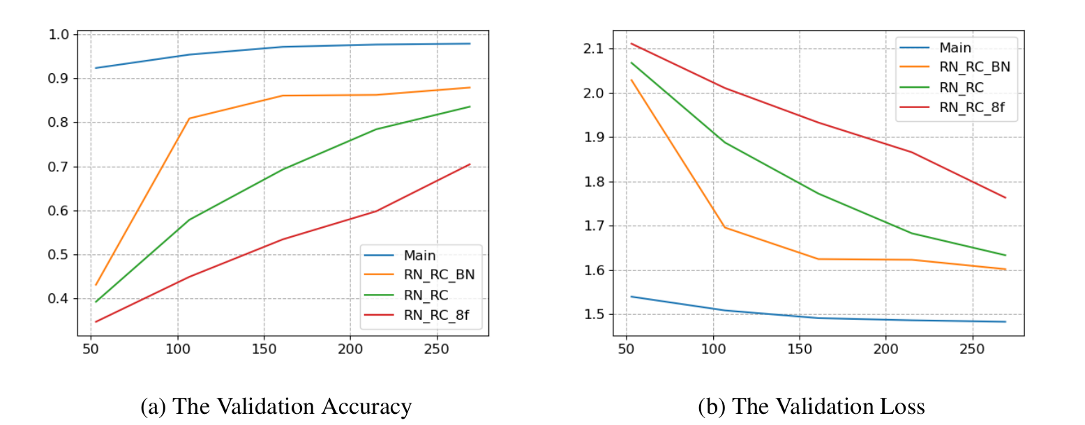
As depicted in figure 6, the final CNN model, referred to as “Main” achieved a validation accuracy of approximately 98% and a validation loss of 1.5. The graph shows that the validation loss initially decreases and then stabilizes. This observation indicates that the CNN model has converged to its optimal state, and further training would only make the model overfit the dataset.

To investigate further, I trained alternative models using various techniques to mitigate overfitting, as shown in figure 6 . Notably, the introduction of random noise and random cropping had a substantial negative impact on performance. This is to be expected given the increase of complexity in the training’s data.

Furthermore, applying batch normalization [4], significantly improved the results. This makes sense because of the normalization process, which helps with mitigating the distribution shift caused by the random noise. It is also worth noting that the model seems to require a minimum of 16 filters, to produce good results, since reducing the number of filters down to 8 hinders performance considerably.

Figure 6: Following abbreviations apply RN = Applies random noise to the images in dataset while training, RC = Random cropping of the images in the dataset while training, BN = Uses Batch norm, 8f = Instead of using 16 filters for the convolutional layer it uses 8 filter.

4. Conclusion & Discussion

This paper provides an overview of Convolutional Neural Network, including their definition and functionality. Additionally, a practical demonstration was conducted aimed to show the capabilities of CNNs and illustrate how a CNN architecture might look like. This serves as an example to showcase the effectiveness of CNNs and provide insight into their architectural structure.

It would have been interesting to explore more alternative models to “Main”. For instance, in section 3.4, I theorized that at least 16 filters are required to achieve good results. However, it is not clear what would happen if I would use slightly fewer filter or doubled the number of filter? Another interesting question is the practical performance of the “RN RC BN” model and how it compares to the “Main” model. Are the introduced transformations realistic and beneficial in real-world applications, or do they hinder the model’s performance?

References:

[1] K. Hornik, M. Stinchcombe, and H. White. Multilayer feedforward networks are universal ap- proximators. Neural Networks, 2(5):359-366, 1989. ISSN 0893-6080. doi: https://doi.org/10.1016/0893-6080(89)90020-8
[2] D. H. Hubel and T. N. Wiesel. Receptive fields, binocular interaction and functional architec- ture in the cat’s visual cortex. The Journal of physiology, 160(1):106, 1962.
[3] S. Ioffe and C. Szegedy. Batch normalization: Accelerating deep network training by reducing internal covariate shift. In International conference on machine learning, pages 448-456. pmlr, 2015.
[4] D. P. Kingma and J. Ba. Adam: A method for stochastic optimization. arXiv preprint arXiv:1412.6980, 2014.
[5] A. Krizhevsky, I. Sutskever, and G. E. Hinton. Imagenet classification with deep convo- lutional neural networks. In F. Pereira, C. Burges, L. Bottou, and K. Weinberger, edi- tors, Advances in Neural Information Processing Systems, volume 25. Curran Associates, Inc., 2012. URL
[6] Y. LeCun, B. Boser, J. S. Denker, D. Henderson, R. E. Howard, W. Hubbard, and L. D. Jackel. Backpropagation applied to handwritten zip code recognition. Neural Computation, 1(4):541- 551, 1989. doi: 10.1162/neco.1989.1.4.541.
[7] Y. Lecun, L. Bottou, Y. Bengio, and P. Haffner. Gradient-based learning applied to document recognition. Proceedings of the IEEE, 86(11):2278-2324, 1998. doi: 10.1109/5.726791.
[8] B. Xu, N. Wang, T. Chen, and M. Li. Empirical evaluation of rectified activations in convolu- tional network. arXiv preprint arXiv:1505.00853, 2015.
[9] M. D. Zeiler and R. Fergus. Visualizing and understanding convolutional networks. In Com- puter Vision-ECCV 2014: 13th European Conference, Zurich, Switzerland, September 6-12, 2014, Proceedings, Part I 13, pages 818-833. Springer, 2014.