Automatic Test Pattern Generation for Printed Neuromorphic Circuits

May 7, 2026 | 1,344 words | 7min read

Paper Title: Automatic Test Pattern Generation for Printed Neuromorphic Circuits

Link to Paper: https://ieeexplore.ieee.org/abstract/document/11049604

Date: 01 July 2025

Paper Type: Neuromorphics, Circuits, Fault Detection

Short Abstract: The paper proposes a new Automatic Test Pattern Generation (ATPG) framework for printed neuromorphic circuits (pNCs) used in printed electronics. These circuits are attractive because they are flexible, cheap, low-power, and suitable for edge AI applications, but they are also highly prone to manufacturing defects.

1. Introduction

Printed Electronics (PE), offers advantages such as flexibility, low cost, customization, and rapid manufacturing through additive printing methods. PE is useful for applications like IoT devices, wearables, RFID tags, smart sensors, and other lightweight electronic systems.

The paper focuses on printed analog neuromorphic circuits (pNCs), which implement analog neural networks directly in hardware. These circuits are well suited to PE because they:

• Process analog signals directly without requiring analog-to-digital converters (ADCs),
• Reduce hardware complexity and device count,
• Match the low-cost, low-density constraints of printed manufacturing.

However, printed analog circuits are difficult to test reliably because PE manufacturing introduces many defects and variations, such as:

• Ink smudging,
• Delamination,
• Void formation,
• Reduced process control compared to conventional silicon fabrication.

Testing is especially challenging because traditional digital ATPG methods do not work well for analog neuromorphic circuits, whose architectures are often custom-designed with hardcoded parameters.

Hence Automatic Test Pattern Generation (ATPG) methods specifically designed for pNCs are needed. Inspired by earlier machine-learning and optimization-based approaches for analog circuit testing, they propose a gradient-based optimization framework that directly targets physical pNCs without relying on neural-network “digital twins.”

The paper’s two main contributions are:

1. Fault analysis and abstraction
   • Identify and group equivalent faults,
   • Remove untestable faults,
   • Improve testing efficiency and fault coverage.
2. Gradient-based test generation
   • Generate optimized test patterns that maximize differences between correct and faulty circuit behavior,
   • Achieve up to 90% fault coverage across nine trained pNC models.

2. Background

2.1 Printed Electronics (PE)

PE uses printing techniques such as inkjet and gravure printing to fabricate flexible electronic circuits with organic or oxide-based semiconductor inks.

• Inkjet printing is additive, precise, and suitable for customized or small-batch production.
• Gravure printing is optimized for large-scale manufacturing.

The paper focuses on n-type electrolyte-gated transistors (nEGTs), which are attractive because they: (1) operate at very low voltages (<1V), (2) consume little power, (3) support flexible and scalable electronics.

Compared to traditional subtractive manufacturing, PE reduces material waste and manufacturing complexity.

2.2 Printed Analog Neuromorphic Circuits (pNCs)

pNCs implement neural-network operations directly in analog hardware for efficient edge AI processing. They are beneficial because they provide:

• low power consumption,
• low cost,
• customization,
• real-time sensor-data processing.

It has two components: (1) resistor crossbars: Crossbar arrays perform the neural-network weighted-sum operation using Ohm’s and Kirchhoff’s laws. Conductance values encode neural-network weights. Extra circuits are added to represent negative weights. Learned parameters correspond to programmable conductances. To implement negative weights separate circuit is needed. (2) Printed Activation Functions: After the weighted sum, outputs pass through printed activation-function circuits such as printed tanh (p-tanh). These circuits introduce nonlinearity, support ANN learning behavior, improve gradient propagation.

Crossbars array learnable parameters i.e. magnitude is the conductiveness and the sign determines if a negative weight circuit is required:

$$ \Theta \in \mathbb{R}^{(M+2)\times N} $$

Crossbar output Voltages:

$$ V^{z} = \left( V^{in} \cdot W \odot \mathbf{1}_{\{\Theta \ge 0\}} \right) + \left( \operatorname{neg}(V^{in}) \cdot W \odot \mathbf{1}_{\{\Theta < 0\}} \right) $$

With the Crossbar Input Voltage:

$$ V^{in} = \left[ V^{1}_{in}, \dots, V^{M}_{in}, 1V, 0V \right] $$

Weight matrix is defined as:

$$ W = |\Theta| \cdot \operatorname{diag} \left( |\Theta|^{\top} \cdot \mathbf{1}_{M+2} \right)^{-1} $$

After the crossbar, the activation fucntion is applied:

$$ V^{out} = \operatorname{ptanh}(V^{z}) $$

Our final output thus is:

$$ V^{out} = \left[ V^{1}_{out}, \dots, V^{N}_{out} \right] $$

2.3 Defects in Additive Printing and Fault Models in Printed

Because PE relies on additive manufacturing, printed circuits are prone to many physical defects, including: broken signal lines, short circuits, ink defects, layer inhomogeneity, nozzle clogging.

The paper categorizes faults into:

• Catastrophic faults: Permanent structural failures such as:
  • stuck-open faults (broken connections),
  • stuck-short faults (unwanted shorts).
• Parametric faults: Variations in component parameters caused by manufacturing imperfections.

2.2 Defects in Additive Printing

In additive printing, we differentiate between:

• Parametric variations: Circuit components do not have exact nominal values but instead exhibit variability.
• Catastrophic faults: These include stuck-open or stuck-short faults, which can be simulated using resistors with very large or very small values (e.g., 100 MΩ and 1 Ω).

3. Methodology

To develop a test pattern generation framework capable of detecting faults in analog neuromorphic circuits, a gradient-based method is used. The goal is to maximize the output discrepancy between fault-free and faulty printable neuromorphic circuits.

Overall methodology:

1. Realistic fault modeling via circuit-level simulations
2. Fault abstraction to reduce test complexity
3. Gradient-based optimization to generate test inputs

3.1 Fault Modeling

The framework models faults in three major pNC components:

• Crossbar conductances,
• Printed tanh activation circuits (p-tanh),
• Negative-weight inverter circuits (p-negative).

The analysis assumes single faults only, since multiple simultaneous faults are unlikely and computationally expensive.

Crossbar Faults

Faults in crossbar conductances are represented with a ternary mask:

$$ M_g \in \{1, 0, \infty\} $$

where:

1 = normal conductance, 0 = open circuit, \(\infty\) = short circuit.

Fault injection is applied to selected conductances within the neural crossbar.

Activation and Inverter Faults

For p-tanh and p-negative circuits, the authors model:

resistor opens/shorts, transistor failures: gate-drain short, gate-source short, drain-source short, gate open.

SPICE simulations generate faulty input-output datasets.

The faulty behavior is approximated using parameterized transfer functions.

For the tanh activation:

$$ p\tanh(V)=\eta_1^T+\eta_2^T\tanh\left((V-\eta_3^T)\eta_4^T\right) $$

For the negative-weight circuit:

$$ pneg(V_z)=-\left(\eta_1^N+\eta_2^N\tanh\left((V_z-\eta_3^N)\eta_4^N\right)\right) $$

The parameters are fitted to SPICE data using nonlinear least squares.

Basically what is done, in SPICE various faults of the circuits are simulated with this a database is created of faults, and this database cna be used to do cruve fitting on the equation above and then we have for every fualt an equation that desrcibes the fault.

3.2 Fault Abstraction

Since exhaustive testing is too expensive, the authors reduce the fault space using two techniques. This means we have too many faults if we go through all possible faults in a neural network, recall that every neuron and every connection can have multiple different faults.

1. Fault Clustering

Faults with similar transfer functions are grouped together as approximately equivalent.

The clustering rule is:

$$ C_k={f_n\mid d(T(f_n),T(c_k))\leq \epsilon} $$

where:

• (T(f_n)) is the transfer function of fault (f_n),
• (c_k) is the cluster centroid,
• (d) is Euclidean distance,
• (\epsilon) is a similarity threshold.

Each cluster is represented by one representative fault, reducing redundancy.

2. Removing Untestable Faults

Faults that never change the circuit’s output are removed.

The maximum output difference is measured as:

$$ \Delta(f_n)=\max_{x\in X}\left|y_{faulty}(x,f_n)-y_{fault\text{-}free}(x)\right|_2^2 $$

If:

$$ \Delta(f_n)=0 $$

the fault is considered untestable and discarded.

This abstraction significantly lowers computational complexity while preserving fault coverage.

3.3 Gradient-Based Test Pattern Generation

After fault abstraction, the framework generates optimized test inputs.

For each fault:

1. Generate 100 random input patterns,
2. Select the best initial candidate,
3. Optimize it using gradient descent.

The objective is to maximize the difference between fault-free and faulty outputs.

Instead of directly optimizing classification disagreement (which uses non-differentiable argmax operations), the method maximizes the Kullback-Leibler (KL) divergence between the softmax output distributions.

The optimization objective is:

$$ L_{KL}(x,f_n)=-\sum_j p_{fault\text{-}free,j}(x)\log\frac{p_{fault\text{-}free,j}(x)}{p_{faulty,j}(x,f_n)} $$

The negative sign allows standard gradient descent optimizers to maximize divergence indirectly.

During optimization:

• gradients are computed through backpropagation,
• inputs are iteratively updated,
• inputs are clipped to the valid voltage range ([0,1]).

A fault is considered detected if the predicted class differs between the fault-free and faulty networks.

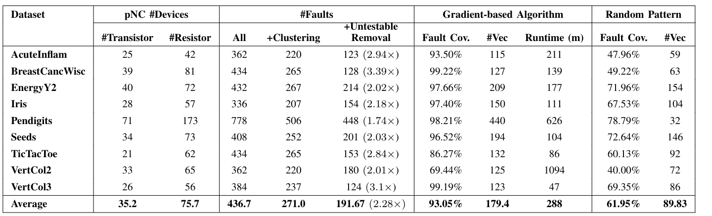
4. Evaluation

The gradient-based algorithm achieved over 90% fault coverage across multiple datasets, significantly outperforming random pattern testing. For example, fault coverage on the BreastCancWisc dataset reached 99.2%, compared to 49.2% with random patterns, albeit with a longer runtime (139 minutes).