Intelligence Processing Units Accelerate Neuromorphic Learning

September 29, 2025 | 779 words | 4min read

Paper Title: Intelligence Processing Units Accelerate Neuromorphic Learning

Link to Paper: https://arxiv.org/abs/2211.10725

Date: 19 Nov. 2022

Paper Type: SNN, Recurrent-SNN, IPU, Training, snnTorch

Short Abstract: This paper presents an extension to the snnTorch library that significantly accelerates the training of spiking neural networks (SNNs) on Intelligence Processing Units (IPUs).

1. Introduction

Artificial intelligence (AI) models have become more popular and larger than ever before. Due to the parallelization provided by GPUs, they have become the dominant platform for training. However, there is a discrepancy: large AI models are trained in data centers consuming hundreds of thousands of watts, while the human brain does not exceed 20 W.

This gap inspires neuromorphic computing, a paradigm that, instead of using artificial neural networks (ANNs), employs spiking neural networks (SNNs). SNNs operate over time: they receive input that is stored in the so-called membrane potential. If the membrane potential exceeds a threshold—also called the action potential—the neuron fires, meaning it emits an output.

Currently, most training of SNNs either (1) happens offline or (2) uses simple plasticity rules. Why don’t SNNs use the highly successful error backpropagation methods from ANNs? There are three main reasons:

1. Because SNNs operate over time, training requires backpropagation through time (BPTT). This means that at every timestep a new network state must be stored, so memory scales linearly with time.
2. Biological neurons are more complex than simple artificial neurons.
3. SNNs are often non-differentiable, which means direct differentiation—required in backpropagation—is not possible.

This paper aims to provide a solution to these problems by presenting an extension for snnTorch that enables training of SNNs using backpropagation.

2. Background

2.1 Training SNNs

When attempting to use backpropagation for SNNs, they encounter three major issues:

• Temporal Credit Assignment: The BPTT learning rule requires storage of all gradients over time, where memory complexity scales with (O(nT)), with (n) being the number of neurons and (T) the simulation time.
• Weight Credit Assignment: Routing gradients from the network’s output back to plastic synapses requires storing the forward data path. Since the gradient of every synapse has an independent pathway, this scales poorly with network size.
• Non-differentiable operations: In leaky integrate-and-fire (LIF) neuron models, a hard threshold is applied to the membrane potential to elicit a spike. This is a non-differentiable operation and thus incompatible with gradient descent.

However, there exist solutions:

1. Temporal Credit Assignment can be addressed using real-time recurrent learning (RTRL) techniques. With this, memory complexity scales as (O(n^3)).
2. Non-differentiable Operations can be handled using surrogate gradients. Here, the non-differentiable function is replaced with a differentiable approximation that preserves similar behavior.
3. Low-cost Inference: While SNN training is expensive, inference is extremely efficient—forward passes are often 2–3 orders of magnitude cheaper than in conventional ANNs.

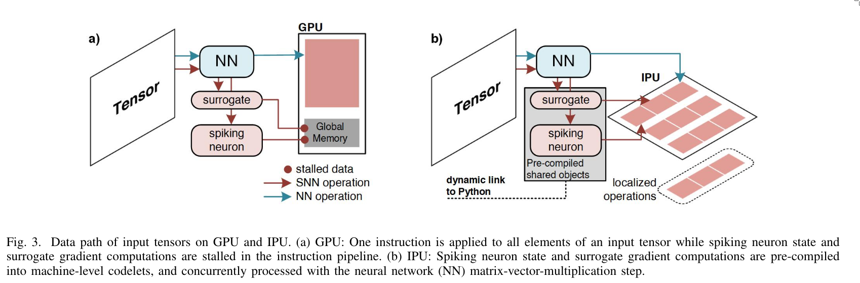
2.2 Intelligence Processing Units

Intelligence Processing Units (IPUs) offer two key advantages over GPUs for training SNNs:

1. Instructions from different network layers can be processed concurrently.
2. MIMD (Multiple Instruction, Multiple Data) processing accelerates applications with irregular and sparse data access without incurring performance degradation.

2.3 Leaky Integrate-and-Fire Neurons

The dynamics of a leaky integrator are as follows:

$$ \tau \frac{du}{dt} = -u + ir $$

where \(u\) is the membrane potential, \(i\) is the input current, and \(r\) is the resistance of the ion channels. The time constant is defined as \(\tau = rc\), with \(c\) the membrane capacitance.

This differential equation can be solved as:

$$ u_t = \beta u_{t-1} + (1 - \beta)i_t $$

where \(\beta = e^{-1/\tau}\) is the inverse time constant of the membrane potential.

When the membrane potential exceeds the threshold \(u_{\text{thr}}\), a spike is generated:

$$ z_t = \begin{cases} 1, & u_t > u_{\text{thr}} \ 0, & \text{otherwise} \end{cases} $$

To introduce a learnable parameter, they replace:

$$ wx := (1 - \beta)i $$

Hence, the update rule becomes:

$$ u_t = \beta u_{t-1} + wx_t - z_{t-1}u_{\text{thr}} $$

2.4 Current-based Leaky Integrate-and-Fire Neurons

In this model, the synaptic input current is modeled as an AMPA receptor with a rapid rise time and gradual decay, which modulates the membrane potential:

$$ i_t = \alpha i_{t-1} + wx_t $$$$ u_t = \beta u_{t-1} + i_t - z_{t-1}u_{\text{thr}} $$

2.5 Recurrent Spiking Neurons

The LIF neuron can be adapted to include an explicit recurrent connection. The output spikes are weighted and fed back into the input:

$$ u_t = \beta u_{t-1} + wx_t - z_{t-1}(v - u_{\text{thr}}) $$

where \(v\) is the recurrent weight.

3. Experiments

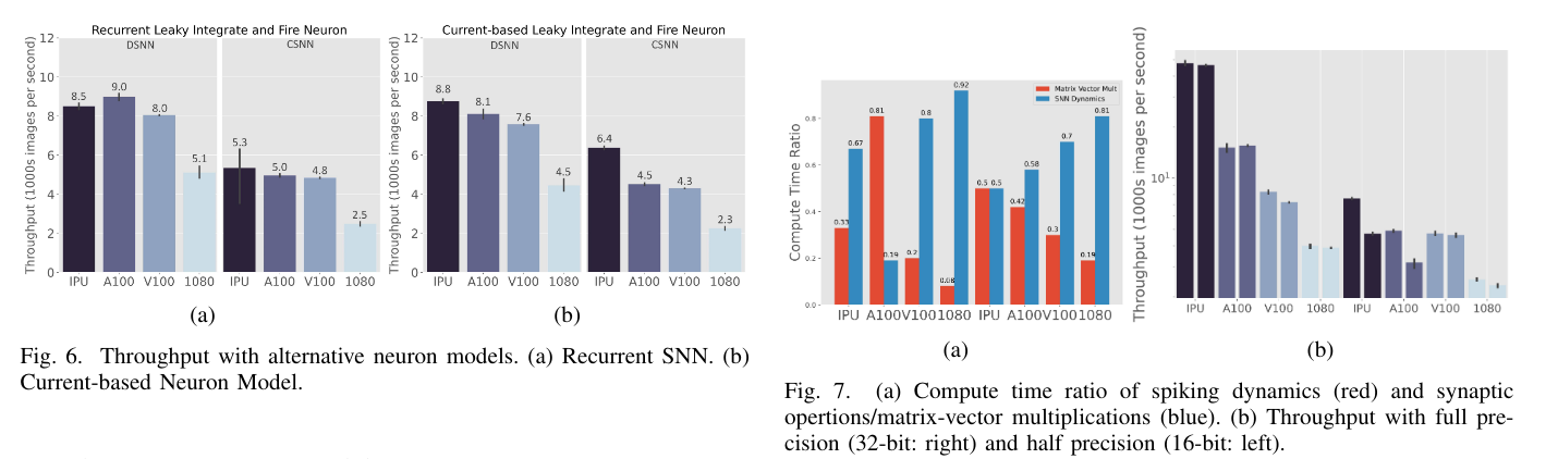
They evaluate different architectures and SNN models, training them on both GPUs and IPUs, and compare their performance. In addition, they investigate:

• Mixed precision training performance.
• Population coding as an alternative to rate coding.

4. Conclusion

They have shown that SNNs can be trained effectively using backpropagation and achieve competitive performance, particularly when trained on IPUs.