Language Model Inversion through End-to-End Differentiation

June 19, 2026 | 1,715 words | 9min read

Paper Title: Language Model Inversion through End-to-End Differentiation

Link to Paper: https://arxiv.org/abs/2602.11044

Date: February 2026

Paper Type: Language Model Inversion, Gradient-based Optimization, Discrete Token Differentiation, Adversarial Prompting

Short Abstract: This paper tackles Language Model Inversion (LMI): given a target output text, find the input prompt that would cause a frozen LM to generate that exact output. The authors propose DLMI (Differentiable Language Model Inversion), which makes LMs end-to-end differentiable by replacing discrete token inputs with continuous distributions over the vocabulary (soft embeddings) and using a Gumbel-Softmax gradient estimator with per-token learnable temperatures. Combined with Teacher Forcing, DLMI achieves near-perfect inversion (LCS ~1.0) even for high-perplexity, non-fluent targets, dramatically outperforming prior methods like GBDA (LCS < 0.2) and REINFORCE (near-zero).

1. The Core Problem

To find the right prompt, one would want to use Gradient Descent, the standard engine of machine learning. Start with a random prompt, pass it through the LM, see how far the output is from the target, and mathematically adjust the prompt to be closer.

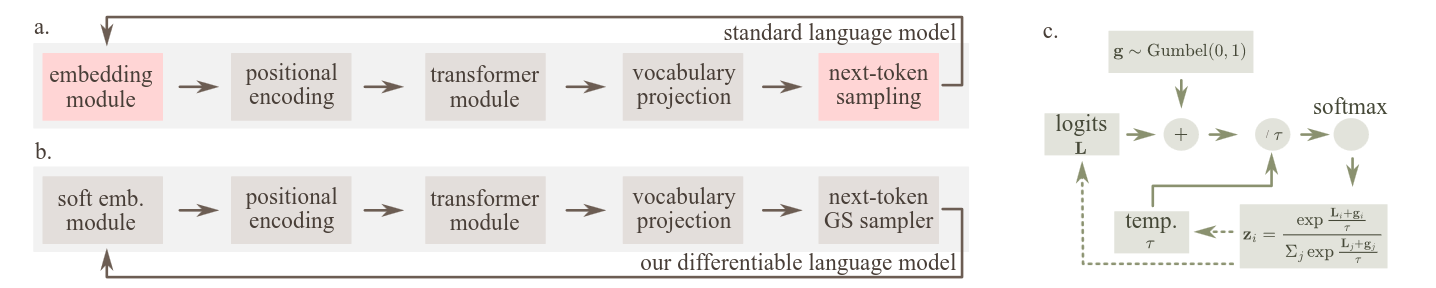
However, standard LMs are not end-to-end differentiable. There are two “barriers” that break the chain of gradients:

1. The Embedding Barrier (Input): LMs don’t read text directly; they look up discrete token indices in an embedding table. Because “looking up a discrete index” is a non-continuous operation, gradients cannot flow backward through it.
2. The Sampling Barrier (Output): When an LM generates the next word, it outputs probabilities over the vocabulary and then picks one (argmax or sampling). Picking a discrete word from a probability distribution is non-differentiable.

The Big Idea: Shift the Perspective

The authors propose a paradigm shift. Instead of viewing an LM as \(f_\theta : V^* \to V^*\) (a function over sequences of tokens), they view it as \(\tilde{f}_\theta : \mathcal{P}^*(V) \to \mathcal{P}^*(V)\), a function over sequences of probability distributions over tokens (SDoT).

Instead of dealing with hard, discrete words, they deal with continuous “soft” probabilities (e.g., 80% apple, 15% orange, 5% banana). This makes the entire process differentiable.

2. Methodology

To make this work, the authors replace the two non-differentiable barriers with differentiable approximations, add a clever temperature trick, and use Teacher Forcing.

2.1 The Soft Embedding Module (Fixing the Input Barrier)

Instead of forcing the input to be a single discrete token, the algorithm treats the input prompt as a sequence of “unnormalized logits” (raw scores for every word in the vocabulary). It passes these through a Softmax function to create a probability distribution over the vocabulary for every position. Then, instead of looking up a single vector, it multiplies the entire embedding matrix \(E\) by this probability distribution:

\[\tilde{x} = \sum_{i=1}^{|V|} p_i \cdot E[i]\]

This creates a “soft embedding”, a weighted average of all word vectors. Because this is just multiplication, gradients can flow backward smoothly.

2.2 Gumbel-Softmax (Fixing the Output Sampling Barrier)

During the LM’s forward pass, when it needs to generate the next token, the authors use the Gumbel-Softmax (GS) gradient estimator. Normally, you add random Gumbel noise to probabilities and take an argmax to sample a discrete token. Gumbel-Softmax replaces the hard argmax with a Softmax with a “temperature” parameter (\(\tau\)):

\[p_{\text{soft}} = \text{softmax}((Z + g) / \tau)\]

where \(g \sim \text{Gumbel}(0,1)^{N \times |V|}\), \(Z\) are the learnable logits, and \(\tau\) is the temperature. This outputs a near-one-hot vector that is continuous and differentiable.

2.3 Learnable, Decoupled Temperature (Key Innovation)

The Gumbel-Softmax relies on a temperature parameter (\(\tau\)):

• Very low \(\tau\): Almost a perfect discrete token, accurate (low bias) but erratic gradients (high variance).
• Very high \(\tau\): A muddy average of all tokens, stable gradients (low variance) but inaccurate (high bias).

The authors’ innovation: instead of a fixed temperature, they make it learnable and decoupled, every token position gets its own independent temperature parameter (\(\phi_i\)):

\[\tau_{\text{eff},i} = \varepsilon + \tau_0 (1 + \tanh(\phi_i))\]

The algorithm automatically learns the optimal balance between stable gradients and accurate discrete tokens for each specific position in the prompt. This is the single most impactful innovation over GBDA (Guo et al., 2021), which uses a fixed global temperature.

2.4 Teacher Forcing

When generating an output of length \(M\), errors can compound. If the model predicts the 2nd word wrong, the 3rd word is doomed. To make optimization efficient, the authors use Teacher Forcing: instead of feeding the model’s own predicted distributions back into itself, they feed the actual ground-truth target (one-hot vectors of \(y\)). This isolates the optimization strictly to finding the input prompt.

They also evaluate a variant without Teacher Forcing (DLMI-TF) to measure its contribution.

2.5 The Optimization Loop

The algorithm runs as follows:

1. Initialize: Random logits \(Z \in \mathbb{R}^{N \times |V|}\) for the prompt (length \(N\)), random learnable temperatures \(\Phi \in \mathbb{R}^N\), frozen target LM, one-hot target output.
2. Forward Pass:
   • Sample Gumbel noise \(g \sim \text{Gumbel}(0,1)^{N \times |V|}\)
   • Compute \(\tau_{\text{eff},i} = \varepsilon + \tau_0 (1 + \tanh(\phi_i))\)
   • Create soft prompt: \(p_{\text{soft}} = \text{softmax}((Z + g) / \tau_{\text{eff}})\)
   • Pass through soft embedding and LM, compare output to target via cross-entropy
3. Backward Pass: Compute gradients w.r.t. \(Z\) and \(\Phi\)
4. Update: Adam optimizer
5. Repeat for \(T_{\text{opt}}\) steps (2048–8192). At the end, take argmax of \(Z^*\) to get the discrete prompt.

3. Evaluation

3.1 Dataset Generation

Previous papers only tried to invert fluent text. The authors created targets of controllable difficulty using a rank parameter \(k\):

• \(k=1\): Most likely tokens, highly fluent, easy to invert.
• \(k=21\): 21st most likely tokens, “weird,” non-fluent text, very hard to invert.
• Targets of length \(M=20\) across \(k \in \{1, 6, 11, 16, 21\}\).

3.2 Baselines

Method	Soft Embeddings	Gradient Estimator	Learnable \(\tau\)	Teacher Forcing
DLMI	✓	Gumbel-Softmax	✓ (per-token)	✓
DLMI-TF	✓	Gumbel-Softmax	✓ (per-token)	✗
GBDA	✓	Gumbel-Softmax	✗ (fixed)	✗
SODA	✓	None (no GS)	N/A	✗
REINFORCE	✗	Policy gradient	N/A	✗

3.3 Key Results

1. DLMI wins decisively: Near-perfect inversion (LCS ratio ~1.0) after 2048 steps across all difficulty levels and both model sizes (SmolLM2-135M and SmolLM3-3B). GBDA (fixed \(\tau\)) plateaued at LCS < 0.2 for difficult targets.

2. Longer prompts are better: \(N=80\) yields vastly better results than \(N=10\).

3. Larger LMs are easier to invert: SmolLM3-3B was easier to invert than SmolLM2-135M, likely because larger models have smoother internal representations.

4. Ablations prove each innovation works:

   • Removing learnable temperature (fixed \(\tau\), like GBDA): LCS drops to < 0.2 for hard targets
   • Removing Teacher Forcing (DLMI-TF): Still strong, but lower sample efficiency
   • Replacing Gumbel-Softmax with REINFORCE: Near-zero LCS

5. Prompt length (\(N\)) matters:

   • \(N=80\): Near-perfect at all difficulty levels
   • \(N=10\): All methods degrade; DLMI still best (LCS 0.6–0.8)

4. Summary

The authors made a Language Model end-to-end differentiable by swapping discrete tokens for continuous probability distributions. By using Gumbel-Softmax to approximate discrete sampling and learning per-token temperatures, they built an algorithm that can reliably reverse-engineer the input prompt for any specific output, even gibberish.

The three key innovations over GBDA are:

1. Per-token learnable temperatures: each position gets its own \(\tau\), adaptively balancing bias and variance
2. Teacher forcing: cleaner gradients via ground-truth token feeding
3. Combined together: DLMI achieves dramatically better convergence than any prior approach

---

Relevance to ATPG and Fault Injection in LLMS

Research context: This work extends ATPG (Automatic Test Pattern Generation) for neural network fault detection to Large Language Models. The core idea is to inject a fault into an LLM and generate an input pattern that maximizes the divergence between healthy and faulty outputs.

Why this paper matters: The fundamental barrier to applying ATPG to LLMs is the discrete token problem. Standard ATPG uses gradient-based optimization to find an input maximizing a divergence signal (KL divergence). In LLMs, the input is a sequence of discrete tokens, gradient descent cannot directly optimize discrete indices. DLMI provides a concrete, well-tested solution to exactly this problem.

Mapping DLMI to ATPG for LLMs:

ATPG Component	DLMI Equivalent	Adaptation Needed
Maximize \(\operatorname{KL}(f_{\text{healthy}} \parallel f_{\text{faulty}})\)	Minimize \(\operatorname{CE}(f(x), \text{target})\)	Replace loss function, KL divergence instead of cross-entropy
Single forward pass (one output)	Autoregressive generation (\(M\) tokens)	Use warmup/generation of faulty output distribution
Input tokens to optimize	Learnable logits \(Z \in \mathbb{R}^{N \times \vert V\vert}\)	Same mechanism, different objective
Fault to detect	Target string \(y\)	No target string, divergence is self-supervised

What needs to be adapted:

1. Loss function: DLMI uses cross-entropy against a known target. For ATPG, the objective is \(\max_x \operatorname{KL}(f_{\text{healthy}}(x) \parallel f_{\text{faulty}}(x))\). The Gumbel-Softmax + learnable temperature machinery transfers directly, but the loss must be replaced with a divergence measure.

2. Teacher forcing applicability: DLMI’s teacher forcing feeds ground-truth tokens. In ATPG there is no ground-truth output. The healthy model’s output distribution could serve as a pseudo-target, or teacher forcing could be omitted.

3. Autoregressive error propagation: A fault at position \(t\) may be masked by errors at earlier positions. DLMI’s learnable temperatures help stabilize early-position gradients.

4. Memory cost: DLMI maintains the same seq_len \(\times \vert V\vert\) logit matrix as GBDA. For Llama 3 8B (\(\vert V\vert = 128\text{K}\), seq_len = 100), this is ~50 MB, acceptable for single-fault scenarios but worth monitoring for batch optimization.

5. Computational cost: DLMI requires 2048–8192 optimization steps per inversion. Each fault location needs its own run, compaction strategies (like K-means in P3) would be essential for scalability.

Why DLMI is preferred over alternatives:

Approach	Why not consider it
Embedding-space optimization (PEZ)	Optimizes in \(\mathbb{R}^{L \times d}\) then projects to nearest token — discretization gap can destroy the fault signal. The KL divergence that detects the fault may rely on directions no real token reaches.
REINFORCE (Geisler et al., 2025)	Policy gradient avoids the \(\vert V\vert\) matrix but has high-variance gradients. For ATPG, where the loss is a KL divergence (not a binary reward), variance may mask small divergence signals.
GBDA (Guo et al., 2021)	Fixed global temperature converges poorly for hard optimization landscapes. DLMI’s learnable per-token temperatures are strictly better.

Open questions:

• Does DLMI’s Gumbel-Softmax converge reliably when the loss is a KL divergence (no fixed target)?
• Can teacher forcing be adapted using the healthy model’s distribution as a reference for the faulty model?
• What sequence length is needed to reliably detect a single fault?
• Can multiple fault locations share a single optimized input (compaction)?

Bottom line: DLMI is the current best candidate for solving the discrete token gradient problem in ATPG-for-LLMs. It provides a differentiable path through discrete token spaces that prior methods (GBDA, PEZ, REINFORCE) cannot match. The remaining work is adapting the loss function from target-matching to divergence-maximization and empirically validating that Gumbel-Softmax gradients remain effective under this new objective.