Learning to learn by gradient descent by gradient descent

March 29, 2025 | 692 words | 4min read

Paper Title: Learning to learn by gradient descent by gradient descent
Link to Paper: https://arxiv.org/abs/1606.04474
Date: 14. June 2016
Paper Type: Meta-Learning, Gradient secent, Neural Network
Short Abstract:
One of the reasons machine learning became so successful is because of a paradigm shift: instead of building algorithms by hand and finely tuning them, we let the computer learn the algorithm from data.
When we look at optimizers like SGD or ADAM, they are still handcrafted. In this paper, the authors attempt to train an optimizer using machine learning that outperforms other optimizers.

1. Introduction

In machine learning, we often express our problem as optimizing an objective function \( f(\theta) \). There are many methods to minimize such a function, but frequently, we use gradient descent-based approaches:

$$ \theta_{t+1} = \theta_t - \alpha_t \nabla f(\theta_t) $$

Many optimization update rules are handcrafted for specific problems, such as deep learning, which deals with high-dimensional, non-convex problems. Examples include SGD, Adagrad, RMSprop, and ADAM, to name a few.

The No Free Lunch Theorem for Optimization states that no single algorithm can perform well on all classes of problems. In other words, only optimizers that specialize in certain types of problems can perform well.

In this paper, instead of using a handcrafted update rule for optimization, the authors propose a learned update rule, called \( g \). An optimization step with this learned optimizer is given by:

$$ \theta_{t+1} = \theta_t - g(\nabla f(\theta_t)) $$

In other words, they train an optimizer, which is then used to optimize a neural network.

2. Learning to Learn Using RNN

Given a neural network with parameters \( \theta \), the function \( f \) we want to optimize, and the parameters of our optimizer’s update rule \( \phi \), we can express the final parameters of the optimized neural network as \( \theta^*(f, \phi) \).

To evaluate whether our learned optimizer is effective, we consider the expected loss:

$$ L(\phi) = \mathbb{E}_f\left[\sum w_t f(\theta)\right] $$

where \( \theta_{t+1} = \theta_t + g_t \) and \( g_t = m(\nabla_t, h_t, \phi) \). Here, \( w_t \) are weights used for regularization, \( m \) is the output of a recurrent neural network (our learned optimizer), parameterized by \( \phi \) (the parameters of our learned optimizer), and \( h_t \) represents the hidden states of the optimizer network.

We minimize \( L(\phi) \) using gradient descent. This is done by sampling a random function \( f \) and applying backpropagation to optimize it.

Simply put, to optimize our optimizer, we need a loss function. This loss function is the expected loss over all possible functions \( f \) that we might want to optimize, which corresponds to the training data we want to fit (e.g., a classification function).

To compute this expected loss, we optimize a neural network for a given function \( f \) using our optimizer, measure the resulting loss, repeat this process for multiple functions \( f \), and average the results.

We then use gradient descent on this calculated loss to improve our optimizer.

3. Experiments

For all experiments, the author used a two-layer LSTM with 20 hidden units per layer. The optimizer network was trained using the loss function described in Section 2 and minimized using the ADAM algorithm, with the learning rate chosen via random search.

The optimizer was compared with contemporary optimization methods such as SGD, RMSProp, ADAM, and Nesterov Accelerated Gradient.

3.1 Benchmarks

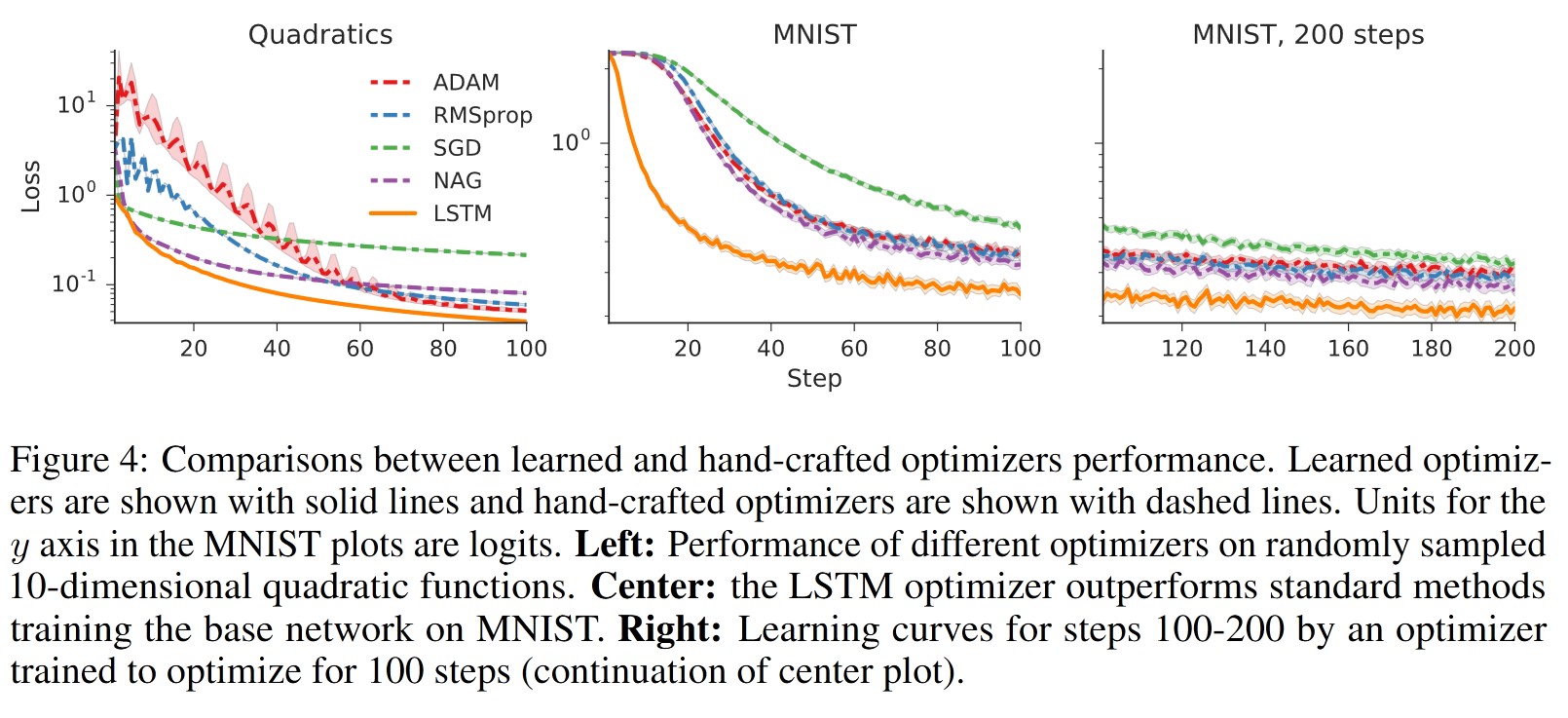
• Quadratic Function: The authors considered synthetic 10-dimensional quadratic functions of the form \( ||W \theta - y||^2 \), where \( W \) is a randomly chosen \( 10 \times 10 \) matrix and \( y \) is a 10-dimensional vector. The optimizer was trained on randomly sampled functions from this family and tested on newly sampled functions.
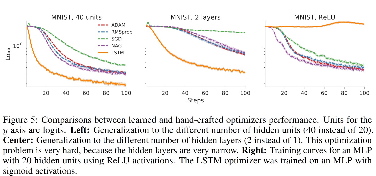
• MNIST: The authors evaluated whether the learned optimizer could train a small neural network on MNIST, experimenting with various modifications to the base network.
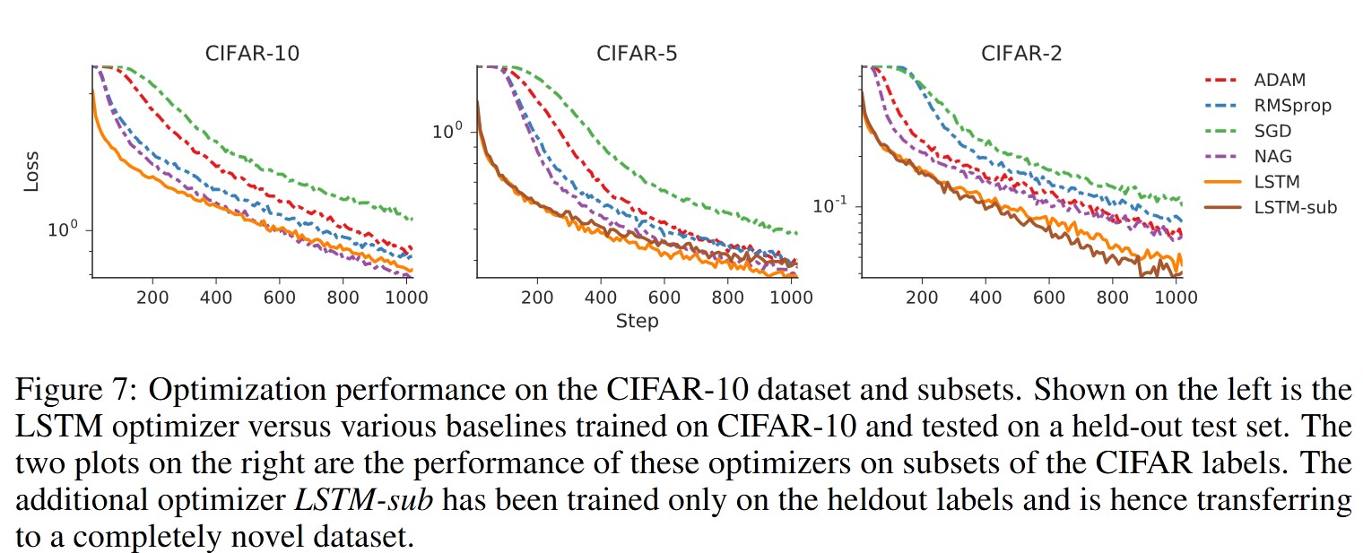
• CNN on CIFAR-10: They trained CNNs on the CIFAR-10 dataset for object classification, using models with both convolutional and feedforward layers.

3.2 Results

4. Conclusion

The experiments confirm that the learned optimizer works well, even in comparison to state-of-the-art optimization methods.