Learning to Optimize

March 29, 2025 | 769 words | 4min read

Paper Title: Learning to Optimize
Link to Paper: https://arxiv.org/abs/1606.01885
Date: 6. June 2016
Paper Type: Meta-Learning, Gradient secent, Neural Network
Short Abstract:
Designing algorithms by hand takes time and requires many iterations. This paper focuses on exploring optimization algorithms that are learned rather than handcrafted.

1. Introduction

Our current approach to designing algorithms is time-consuming and difficult. It requires a mix of intuition and theoretical/empirical insight, followed by performance analysis and iterative refinement. Thus, automating this process would be beneficial.

This paper focuses on automating the design of optimization algorithms, such as gradient descent, momentum, and L-BFGS.

A better optimization algorithm is learned by observing its execution. Therefore, the problem can be framed as a reinforcement learning problem. In this framework, every policy corresponds to a particular optimizer. An optimizer that converges quickly is rewarded. The problem then reduces to finding the optimal policy. We distinguish between the “learner” (the model trained to execute a certain task) and the “policy” (the optimizer algorithm used to train the learner).

2. Method

2.1 Preliminaries

In reinforcement learning, the learner takes an action at each time step, which impacts the environment and receives feedback in the form of a reward. The objective of the learner is to maximize this reward by choosing the best possible actions.

We can model a reinforcement learning problem with the help of a Markov decision process (MDP), where the nodes represent the states the environment can be in, and the connections between nodes represent the actions the learner can take in each state.

The goal is to learn a stochastic policy that minimizes the cumulative cost:

$$ \pi^* = \arg\min_{\pi} \mathbb{E}_{s_0, a_0, s_1, \dots, s_T} \left[ \sum_{t=0}^{T} \gamma^t c(s_t) \right], $$

where \(\gamma\) is the discount factor.

Finding the best policy is known as the policy search problem. To improve generalization, we want to parameterize the policy. While finding the best policy is intractable, we can approximate it.

Guided policy search is an algorithm used to find an approximate best policy, and this is the method employed in this paper to find the policy.

2.2 Formulation

Below is the structure of an optimization algorithm. The algorithm starts from a random point and iteratively updates its current location using a computed step vector from some policy \(\pi\), based on the current and past locations.

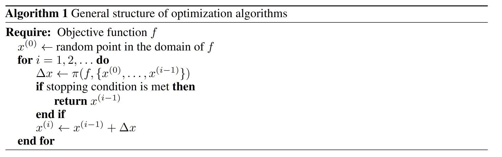
Every optimizer can be expressed using the framework above. Different optimizers differ in their choice of \(\pi\). For example, gradient descent can be expressed as follows:

$$ \pi \left( f, \{ x^{(0)}, \dots, x^{(i-1)} \} \right) = -\alpha \nabla f(x^{(i-1)}), $$

Gradient descent with momentum is formulated as:

$$ \pi \left( f, \{ x^{(0)}, \dots, x^{(i-1)} \} \right) = -\alpha \left( \sum \alpha^{i-1-j} \nabla f(x^{(i-1)}) \right). $$

Thus, by choosing \(\pi\) appropriately, we can learn an optimization algorithm.

We can interpret a given policy as executing multiple actions in an MDP, where the state in the MDP corresponds to our current location in the objective function, and the action is the step vector of our optimization algorithm.

To learn this policy \(\pi\), we use reinforcement learning. For this, we need to define the cost function, which penalizes slow convergence. We define the cost based on the current location in the objective function.

2.3 Discussion

Learning the optimizer can be interpreted as minimizing the a priori assumptions made about the objective functions. This is because, when we hand-design algorithms, we make various assumptions about the loss landscape.

Another advantage of this method is that there are no hyperparameters to tune, as the policy automatically combines the step direction and step size.

2.4 Implementation Details

The authors track the previous \(H\) time steps of the optimizer, using \(H = 25\). The state space encodes the following information per step:

• Current location.
• Change in objective value at the current location relative to the most recent location.
• Gradient of the objective function.

To model the policy, they use a neural network consisting of a single hidden layer with 50 neurons and softplus activation functions.

For training, they perform 20 trajectories with 40 time steps for each objective function in the training set.

3. Experiments

3.1 Setup

The optimizer is trained on various classes of objective functions:

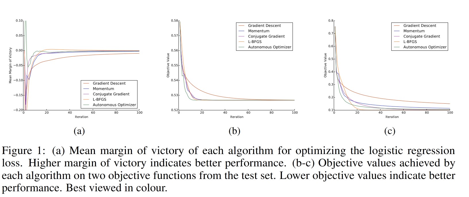
• Logistic regression: The training set consists of examples of logistic regression problems. They use 90 objective functions in their dataset.
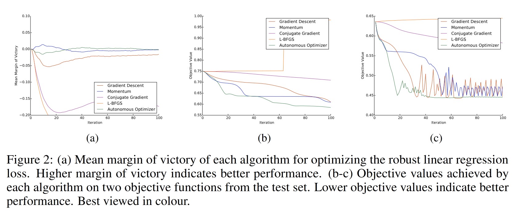
• Robust linear regression: The problem of linear regression using a robust loss function.
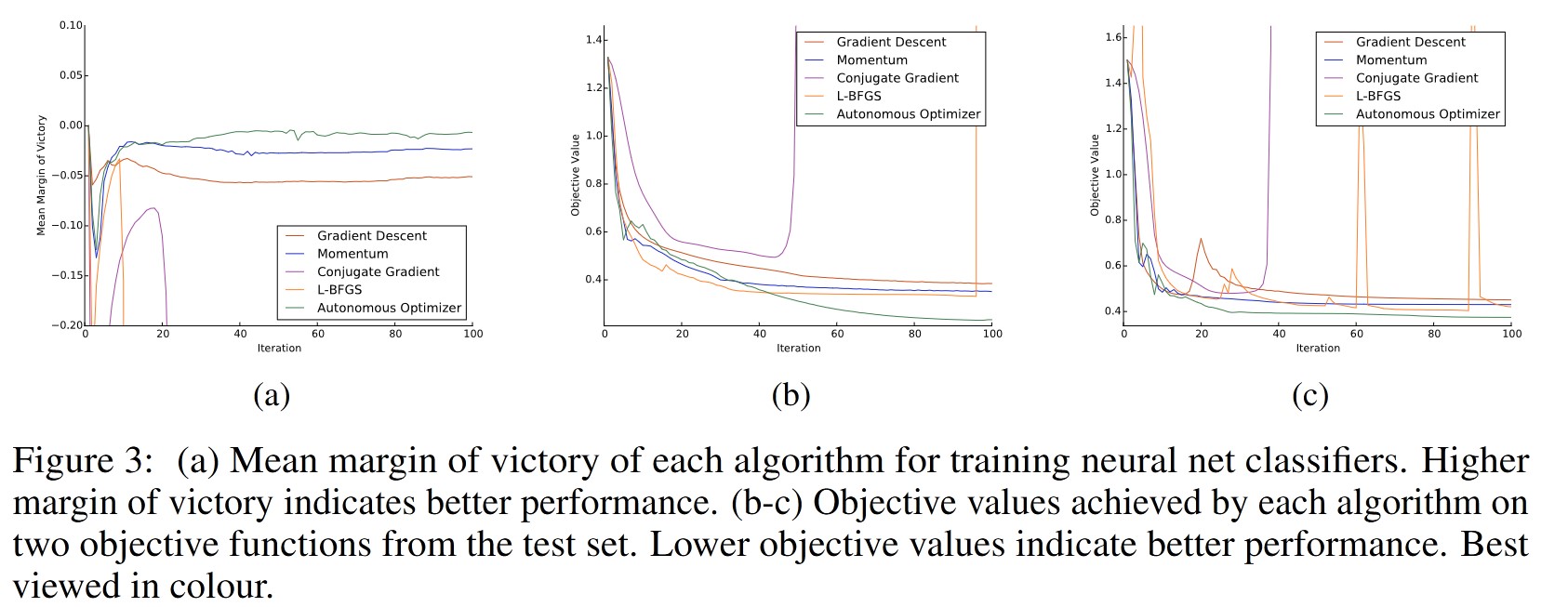
• Neural net classifier: Training a small neural network to classify data.

The optimizer is compared to commonly used optimizers in machine learning.

3.2 Results

4. Conclusion

The learned optimization algorithm works and performs as well as or better than other state-of-the-art optimizers.