Learning to Optimize Neural Nets

March 30, 2025 | 565 words | 3min read

Paper Title: Learning to Optimize Neural Nets
Link to Paper: https://arxiv.org/abs/1703.00441
Date: 1. March 2017
Paper Type: Meta-Learning, Gradient secent, Neural Network
Short Abstract:
This is a follow-up paper to Learning to Optimize, in which reinforcement learning was used to learn an optimizer. In this paper, the authors apply this framework to learning optimizers for shallow neural networks.

1. Introduction

The philosophy of machine learning is that, in general, algorithms learned from data perform better than handcrafted algorithms. This idea can also be applied to the algorithms used for learning—specifically, optimization algorithms.

The paper Learning to learn by gradient descent by gradient descent focuses on learning optimization algorithms for training models on specific tasks. These task-dependent optimization algorithms are trained in a supervised manner.

In contrast, Learning to Optimize introduces a task-independent learned optimization algorithm. It demonstrates that any optimization algorithm can be framed as a reinforcement learning problem with the following general structure:

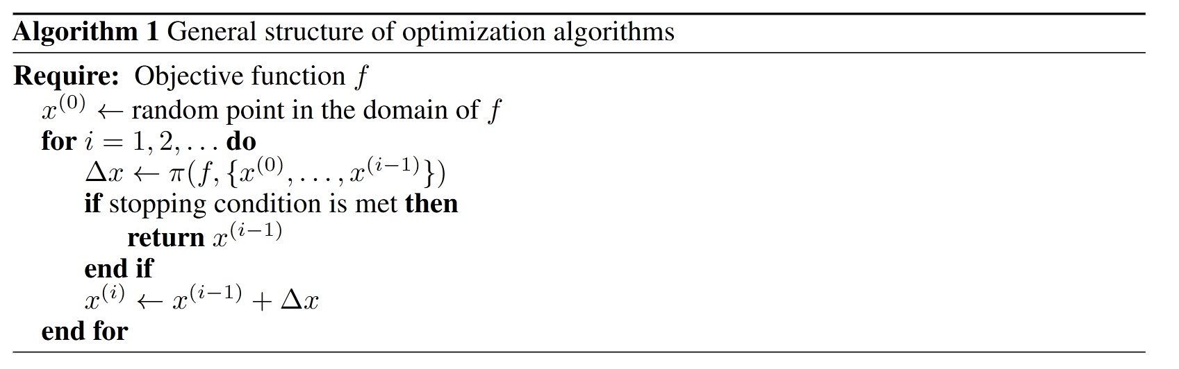
In each iteration, the algorithm takes a step $\Delta x$ and uses it to update the current iterate $x^i$. In handcrafted optimization algorithms, the update $\Delta x$ is calculated using a fixed formula, depending on the objective function, the current iterate, and past iterates.

Different choices of $\pi$ lead to different optimizers. The goal of the paper is to train an optimizer suitable for training shallow neural networks.

2. Learning to Optimize

In the Learning to Optimize framework, we have a set of training objective functions $f_1, ..., f_n$. We are also given an initial iterate $x^0$ and a meta-loss $L$, which takes an objective function $f_i$ and a sequence of iterations $x^0,...,x^n$ produced by an optimization algorithm. The goal is to learn an algorithm $A^*$ that minimizes

$$ \mathbb{E}[L(f, A^*(f, x^0))] $$

The objective function represents the loss function for training a particular base learner (neural network) on a specific task. Thus, different objective functions correspond to training the base learner on different tasks.

We can model this as a reinforcement learning problem, where the task is to find an optimal policy. The state consists of the current iterate $x^t$ and features $\phi$ that depend on the history of iterates, the gradient of the objective function, and the objective function value.

The policy is modeled as a recurrent neural network, which takes as input the observation features and the previous state, then outputs an optimization step to take.

To learn the best possible policy, guided policy search (GPS) is used. Learning high-dimensional optimization algorithms is challenging for reinforcement learning due to the curse of dimensionality. Additionally, GPS has a running time that scales cubically with the dimensionality of the state space. To address this, the authors use convolutional GPS.

For input features in the optimization algorithm, they use the following, which represent the average of recent iterates, gradients, and objective values, respectively:

$$ \overline{x(i)} := \frac{1}{\min(i+1,3)} \sum_{j=\max(i-2,0)}^{i} x(j) $$$$ \overline{\nabla \hat{f}(x(i))} := \frac{1}{\min(i+1,3)} \sum_{j=\max(i-2,0)}^{i} \nabla \hat{f}(x(j)) $$$$ \overline{\hat{f}(x(i))} := \frac{1}{\min(i+1,3)} \sum_{j=\max(i-2,0)}^{i} \hat{f}(x(j)) $$

3. Experiments

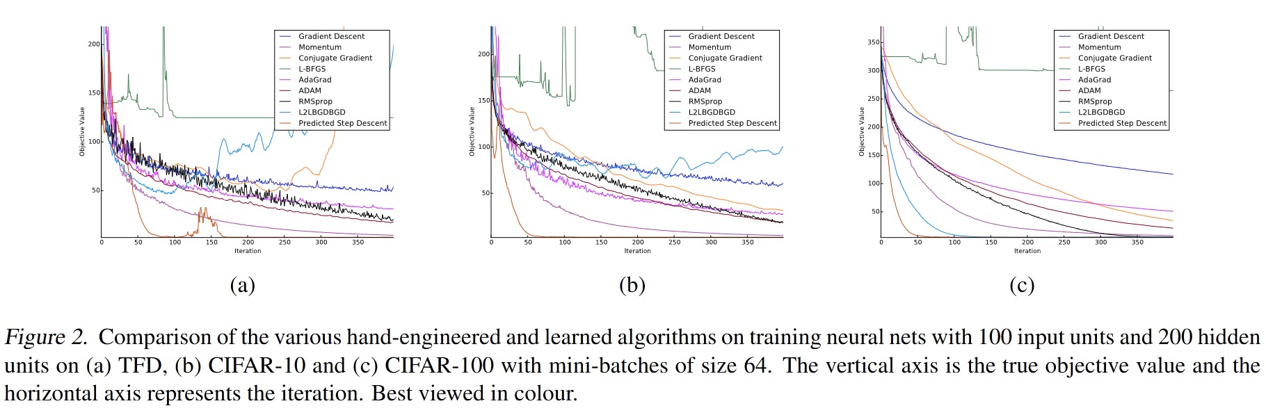
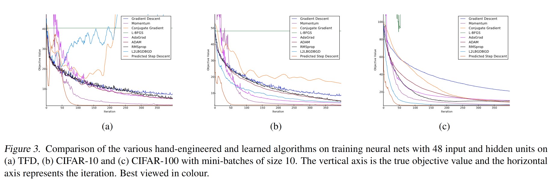
The authors meta-trained a two-layer neural network with 48 inputs, 48 hidden units, and 10 output units on a normalized version of MNIST. The optimizer network is modeled using an RNN with a single layer of 128 LSTM units.

The learned optimization algorithm is evaluated on the Toronto Face dataset, CIFAR-10, and CIFAR-100.

4. Conclusion

The learned optimization algorithm generalizes to other problems involving training neural networks and is robust to changes in the neural network architecture.