Power-Aware Training for Energy-Efficient Printed Neuromorphic Circuits

July 1, 2025 | 973 words | 5min read

Paper Title: Power-Aware Training for Energy-Efficient Printed Neuromorphic Circuits
Link to Paper: https://ieeexplore.ieee.org/document/10323917
Date: 22. November 2023
Paper Type: Neuromorphic Computing, SNN, Printed Electronics, Circuit Design
Short Abstract:
In this paper, the authors develop a neuromorphic chip model that can be optimized for both accuracy and power usage. Their experiments reveal that the model achieves a 2× reduction in power consumption while maintaining 95% accuracy.

1. Introduction

See Analog Printed Spiking Neuromorphic Circuit and Highly-Bespoke Robust Printed Neuromorphic Circuits for a more general introduction.

This paper focuses on optimizing the power usage of neuromorphic chips. By leveraging SPICE simulation, the authors build a power consumption approximation model that is fully differentiable and can therefore be incorporated into the loss function for backpropagation.

2. Background

See Analog Printed Spiking Neuromorphic Circuit and Highly-Bespoke Robust Printed Neuromorphic Circuits for a more.

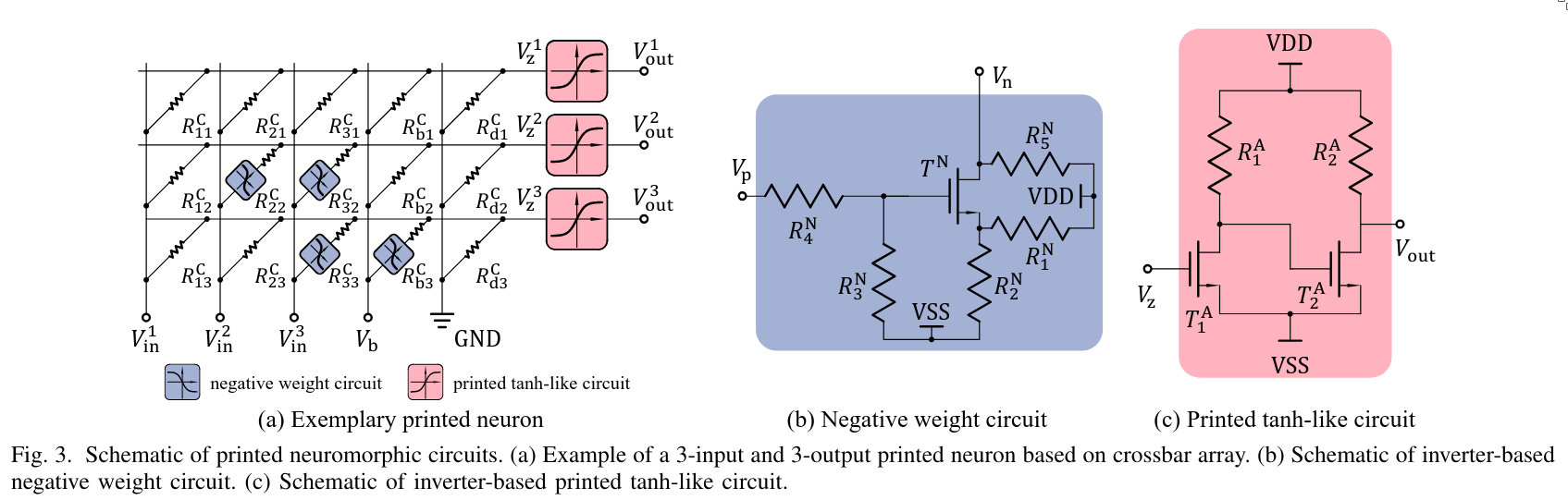
Very broadly, artificial neural networks (ANNs) use weighted sums and non-linear activation functions. Using Kirchhoff’s law, it can be observed that placing the input synapses—which deliver voltage to the target neuron—in parallel results in a summing effect. Additionally, by placing resistors between the synapses (which act like weights in a neural network), it becomes possible to implement a circuit-level equivalent of a weighted sum operation.

In their design, the authors use a crossbar array to implement this functionality. One disadvantage of such arrays is that, since they operate only with resistive elements, representing negative weights becomes challenging. To address this, a negative weight circuit is introduced—this circuit models a negative weight relationship. A negative weight circuit can be implemented using the hyperbolic tangent (tanh) function, which also serves as the activation function.

Together, this setup implements a single neuron, as illustrated below.

By connecting multiple of these neurons together, they construct a neural network. Importantly, these networks do not employ reconfigurable components to enable on-device training during usage.

Instead, they are designed and optimized off-device at the software level. This is not a limitation, as they use Printed Analog Neuromorphic Circuits (PE), which are low-cost and allow for on-demand fabrication.

They refer to this architecture as a printed neural network (pNN). The pNN is trained on a target dataset, from which the optimal physical parameters (e.g., resistor strengths in the circuit) are derived for the subsequent fabrication process.

The pNN consists of a crossbar array denoted \(\Theta\), with which the output voltage can be expressed as:

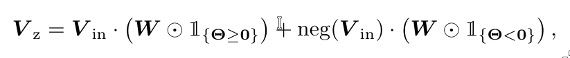
Here, \(V_z\) represents the weighted sum of the input voltages, with \(V_{\text{in}}\) being the input voltages, and \(\odot\) denoting the element-wise product. An indicator function is used to differentiate between negative and positive weights—negative weights require the use of the negative weight circuit.

The final output of the neuron is then obtained by applying the activation function:

$$ V_{\text{out}} = \text{ptanh}(V_z) $$

3. Methodology

3.1 Modified Power-Efficient Circuit Structure

The original crossbar design, as shown in the first figure, uses multiple negative weight circuits. This is due to the use of a simple crossbar structure. However, this approach is suboptimal in terms of power efficiency—it would be better if each input required only a single use of the negative weight circuit.

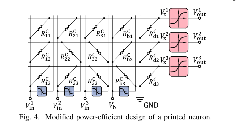
As you can see, they use one negative weight circuit for every input. As a result, each input requires two wires: one for the “normal” (positive) weight and one for the negative weight. If a positive weight is needed, the resistor is connected to the positive wire; if a negative weight is required, the transistor is connected to the wire corresponding to the negative weight.

3.2 Power Consumption Model

Because the goal is to optimize the model with respect to power consumption, the authors propose a fully differentiable power consumption model. This allows the power consumption to be incorporated into the loss function, enabling the use of backpropagation to optimize the model parameters accordingly.

Importantly, the following expression represents the power consumption model for a single neuron in their circuit, as described in the previous section.

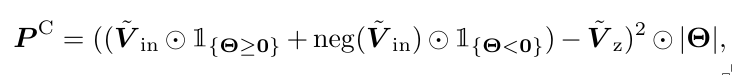
For the power consumption of the crossbar, the model uses the standard formula:

$$ P = \frac{\Delta V^2}{R} = \Delta V^2 \cdot g $$

where \(\Delta V\) is the voltage difference, \(R\) is the resistance, and \(g = \frac{1}{R}\) is the conductance.

Thus

Estimating the power consumption of the activation function is more challenging due to its nonlinearity. Instead of calculating it exactly, the authors approximate it using a neural network. They call this approach Surrogate Power Consumption Models for Nonlinear Circuits.

To do this, they rebuild their circuit in SPICE software and simulate its power behavior, generating a dataset consisting of pairs \((\text{parameters}, \text{power usage})\).

This dataset is then used to train an artificial neural network (ANN). As a result, they obtain an ANN that takes the circuit parameters (such as resistor strengths) as input and outputs an approximation of the circuit’s power consumption.

3.3 Power Estimation for a Printed Neuron

To obtain the final power estimation for a single neuron, the authors use the formula:

$$ P = P^C + N^N \cdot P^N + N^A \cdot P^A $$

where \(P^C\) is the power consumption of the positive weights in the crossbar; \(N^N\) and \(N^A\) denote the number of negative weight circuits that require special treatment due to the use of the tanh function; and \(P^N\) and \(P^A\) are the estimated power consumptions obtained from the surrogate power model.

3.4 Power-Aware Training

Typically, artificial neural networks use cross-entropy loss. However, for printed neural networks (pNNs), the loss function is slightly modified (see the paper for details) to account for minimal distinguishable voltages by employing a hinge loss.

The final loss function combines classification accuracy and power consumption:

$$ L' = (1 - \alpha) \cdot L + \alpha P $$

4. Experiment

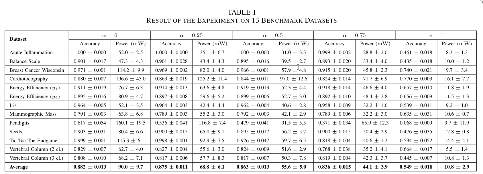
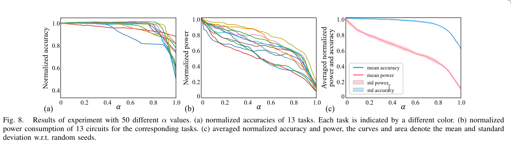
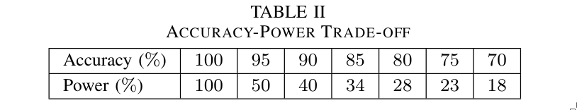
5. Conclusion

Both the strategy of reducing the number of negative weight circuits and the use of power-aware training contribute to a substantial power reduction (2x) while maintaining 95% of the original accuracy.