Highly-Bespoke Robust Printed Neuromorphic Circuits

June 30, 2025 | 1,629 words | 8min read

Paper Title: Highly-Bespoke Robust Printed Neuromorphic Circuits
Link to Paper: https://publikationen.bibliothek.kit.edu/1000156490
Date: 06. March 2023
Paper Type: Neuromorphic Computing, SNN, Printed Electronics, Circuit Design
Short Abstract:
In this paper, the authors propose to expand P-SNN with learnable activation functions and variation-aware training that accounts for manufacturing differences in the printing method

1. Introduction

Modern devices: such as small robots, IoT devices, and wearable technology; all require power-efficient and low-cost solutions. These requirements are often not met by traditional silicon-based circuits.

Printed electronics (PE) offer a promising alternative. They are cheaper to produce, require fewer fabrication steps and less equipment, and can be implemented on flexible materials.

Furthermore, with the ever-increasing popularity and demand for machine learning, neuromorphic computing has become increasingly interesting. The fundamental operations in neuromorphic computing are the weighted-sum operation and the activation function.

In circuitry, the weighted-sum operation has been implemented using resistor crossbars.

There have been many works on neuromorphic chips; however, these have almost exclusively focused on using resistors as learnable parameters.

In this paper, the authors propose to also learn the non-linear operation—i.e., the activation function. In addition, they introduce variation-aware training that accounts for the manufacturing imperfections of printed electronics, where each component can have slightly different dimensions and characteristics.

2. Background

Printed Manufacturing

• Advantages:
  • Compatible with many different materials
  • Requires less and cheaper equipment
  • Circuit fabrication is ultra low-cost
  • Printable components can be easily modified
  • The high flexibility of printed electronics is leveraged to enable learnable activation functions
• Disadvantages:
  • Large feature size and low integration density
  • High fabrication variability
  • The authors address this variability by using variation-aware training, which allows the model to learn despite these imperfections

Analog Neuromorphic Circuits

• Analog circuits have an advantage over digital ones due to their lower component requirements.
  • For example, a 3-input, 1-output, 4-bit digital neuron may require hundreds of transistors, while an analog approach can achieve similar functionality with fewer than ten components.
• Disadvantage: Analog circuits are more prone to errors.
• These circuits are often realized using resistor crossbars, where the inputs to a single neuron are multiple voltages, each scaled by a resistor that represents a weight.

Activation Function

• A tanh-like activation function can be approximated in circuitry using two inverters, following the formula: $$ V_a = ptanh(V_z) = n_1 + n_2 \cdot \tanh((V_z - n_3) \cdot n_4) $$ where:
  • \(V_z\): input voltage
  • \(V_a\): output voltage
  • \(n = [n_1, n_2, n_3, n_4] \): a parameter vector that modifies the shape of the function
• Importantly, these parameters \(n\) are not tied to the physical components of the circuit. They are learnable and can be tuned during training.

Negative Weight Circuits

• Weights are typically formed via the resistor crossbar. However, since resistors cannot produce negative values directly, implementing negative weights in neural networks requires a workaround.
• To address this, a negative weight circuit is used. This circuit reuses the previously defined tanh-based function to reverse the input-output relationship, saving on hardware complexity.
• Notably, this does not make the voltage itself negative; rather, it changes the relationship between the input and the output:
  • For a regular tanh-like activation (ptanh):
    • Low input → Low output
    • High input → High output
  • For the negative weight function (inv):
    • Low input → High output
    • High input → Low output
• The signal remains in the positive voltage range, but the behavior simulates a negative weight.

3. Methodology

3.1 Modeling of Nonlinear Circuits

We previously defined the tanh-like activation function as:

$$ V_a = ptanh(V_z) = n_1 + n_2 \cdot \tanh((V_z - n_3) \cdot n_4) $$

However, the parameters \(N = [n_1, n_2, n_3, n_4]\) are not directly tied to physical circuit components. While we can use backpropagation to learn these parameters during training, we do not know how to map them to actual hardware—specifically, how to set physical components like resistors to implement the desired tanh behavior.

To solve this, we aim to learn a differentiable mapping:

$$ \omega \mapsto N $$

where $\omega$ represents physical parameters of the circuit (e.g. resistor values). This mapping allows us to learn physical circuit parameters via gradient descent.

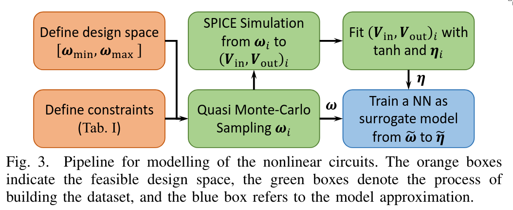
To build this mapping, we proceed as follows:

1. Determine Physical Constraints Printed electronics cannot support arbitrary circuits due to physical limitations. We must identify and respect these constraints when designing our components.

2. Dataset Generation To learn the mapping \(\omega \mapsto N\), we need training data. This is created as follows:

   • We model the tanh-like activation circuit using SPICE simulation software.
   • We systematically vary the physical parameters (e.g., resistor strengths) using Quasi Monte Carlo sampling, while keeping the input voltage constant.
   • For each configuration, we record:
     • Input voltage \(V_{in}\)
     • Physical parameters \(\omega\)
     • Output voltage \(V_{out}\) This results in a dataset that captures how physical components relate to the behavior of the activation function.

3. Train Surrogate Activation Function Based on this dataset, we train an artificial neural network (ANN) to act as a surrogate model of the activation function.

   • Since the mapping from physical parameters to function behavior is differentiable, we can use backpropagation during training.
   • This surrogate model replaces expensive SPICE simulations during training.
   • SPICE itself is not differentiable, and running simulations during training would be prohibitively slow.

4. Training and Deployment

   • During model training, we construct a standard neural network architecture that includes learnable activation functions modeled by the surrogate ANN.
   • These learnable activation functions follow the tanh-like form: $$ V_a = ptanh(V_z) = n_1 + n_2 \cdot \tanh((V_z - n_3) \cdot n_4) $$
   • Once the model is trained, we use the learned \(N\) parameters and apply our trained mapping \(\omega \mapsto N\) in reverse to determine the physical components needed for each activation function in the printed circuit.

One might ask: why do we need to learn the mapping from weights to physical components in the first place? Shouldn’t there be a simple formula to calculate this directly?

The answer is yes, for simple components — for example, in a basic crossbar structure, the mapping is straightforward and can be calculated analytically. However, for more complex components like a tanh-shaped activation function, which consists of multiple circuit elements, the mapping becomes much more complicated. In such cases, one would need to solve a system of nonlinear equations, which is computationally slow and often impractical.

Therefore, using a learned approximation (surrogate model) is a more efficient and scalable solution.

3.2 Constraints

There is one more important detail in the pipeline—namely, how the constraints identified in phase 0 are incorporated during training.

To respect these physical constraints, the model does not learn absolute values for the circuit parameters. Instead, it learns the ratios that satisfy the inequality constraints defined by the fabrication process.

To implement this:

• The learnable parameters are normalized to the range (0, 1) using a sigmoid function.
• During deployment, these normalized parameters are denormalized to produce actual physical values that can be used in printed circuits.

This ensures that the learned values remain within feasible, printable ranges while still being optimized via gradient-based methods.

3.3 Variation-Aware Training

Variation-aware training refers to accounting for fabrication variability: that is, the random errors that naturally occur when printing circuit components.

To model this:

• The physical parameters \(\theta\) are treated as stochastic variables, rather than fixed values: $$ \theta \sim p(\theta) $$
• This introduces a noise term \(\epsilon\), modeling the fabrication error, so that: $$ \hat{\theta} = \theta + \epsilon $$
• Consequently, the loss function must also change: instead of being deterministic, it becomes an expected loss over the distribution of possible parameter values: $$ \mathcal{L} = \mathbb{E}_{\theta \sim p(\theta)}[\text{Loss}] $$

4. Experiments

4.1 Setup

• An ablation study was conducted to assess the effects of:
  • Learnable activation functions, and
  • Variation-aware training
• A total of 13 different benchmark datasets were used.
• The pNN architecture consisted of:
  • An input layer,
  • A hidden layer with 3 neurons, and
  • An output layer
• Optimization was done using the Adam optimizer.
• Early stopping was employed with a patience of 5000 epochs to avoid overfitting.

4.2 Results

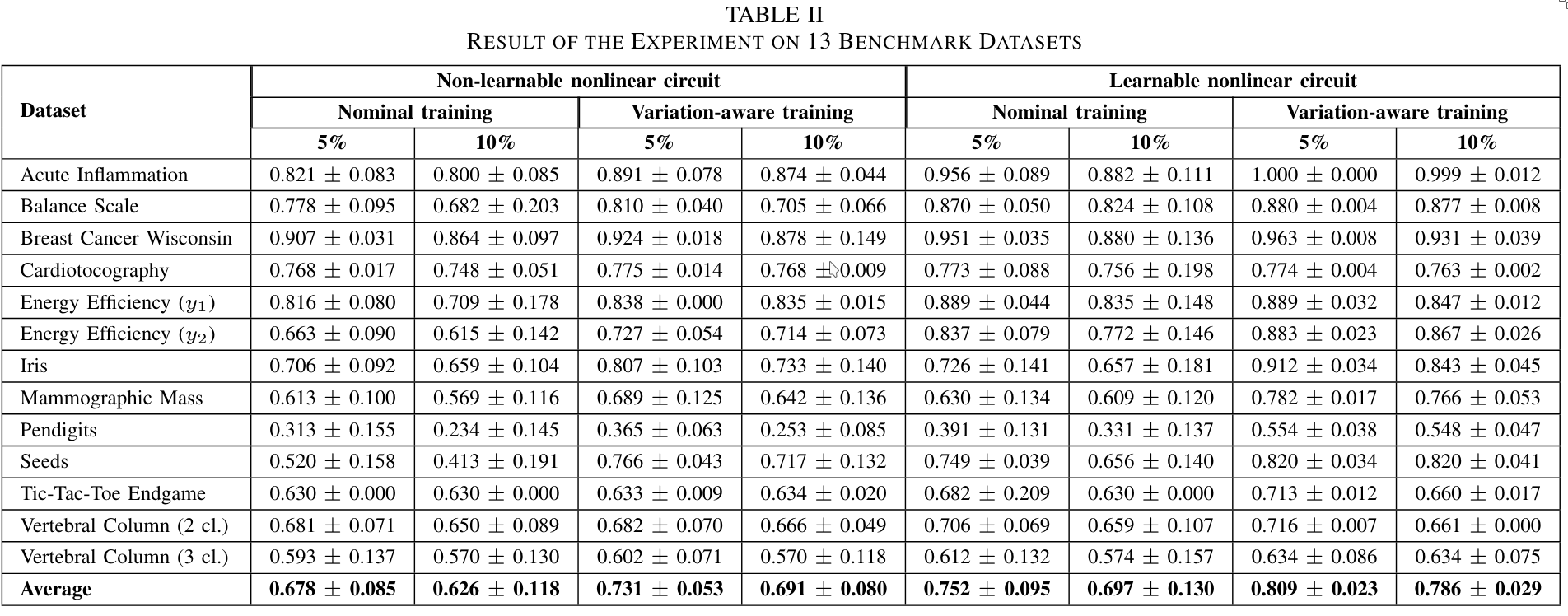
5. Conclusion

Both the variation-aware training and the learnable activation functions substantially increase accuracy.

---

My Thoughts

I am a bit unsure about exactly how they train the weights of the model, specifically the weights in the P-SNN circuit, which correspond to the strength of the resistors in the crossbars. My best guess is that they do it similarly to Hardware Efficient Weight-Binarized Spiking Neural Networks, which is from the same authors.

Also, when the paper refers to neuromorphic, it specifically means three things (1) Analog computation, (2) Neural network-based structure, (3) Physically implemented as a printed circuit. It does not imply the use of spiking neural networks (SNNs) or any other biologically inspired models. So, in this paper, the term “neuromorphic” is used in a very specific and narrow way: analog neural networks physically realized in hardware. Personally not a fan of this definition.

I think variation-aware training is a good idea. However, I’m more skeptical about learnable activation functions. There is a reason why larger neural networks usually use the same activation function throughout:

• We risk over-parameterizing, causing the model to lose generality.
• It adds another hyperparameter that needs to be optimized, increasing resource demands.
• As long as the activation function doesn’t have (1) vanishing gradient problems (e.g., sigmoid), (2) dead zones (e.g., ReLU), or (3) high computational complexity (e.g., tanh), the choice of activation has limited impact.

For example, does the model truly get better because of the learnable activation function, or just because it implicitly has more parameters? I suspect a similar accuracy improvement could be achieved simply by using more neurons.

The question then becomes: what is computationally cheaper?