RWKV: Reinventing RNNs for the Transformer Era
June 26, 2025 | 1,676 words | 8min read
Paper Title: RWKV: Reinventing RNNs for the Transformer Era
Link to Paper: https://arxiv.org/abs/2305.13048
Date: 22. May 2023
Paper Type: LLM, Architecture
Short Abstract:
RWKV is a technique designed to replace self-attention in recurrent neural networks (RNNs). It is used to train a 14-billion-parameter model that achieves performance competitive with traditional transformer-based large language models, while requiring significantly fewer computational resources to train.
1. Introduction
Deep learning has been highly successful, particularly in the domain of natural language processing (NLP), with the rise of the transformer architecture. Before transformers became popular, recurrent neural networks (RNNs) were the dominant architecture for language-related tasks. However, RNNs suffer from issues such as vanishing gradients, lack of parallelizability, and limited scalability.
Transformers, while powerful, have their own limitations. The self-attention mechanism has quadratic complexity, is memory-intensive, and has a fixed context size, making training computationally expensive.
To address these issues, the authors propose a new architecture called Receptance Weighted Key Value (RWKV), which combines the strengths of RNNs and transformers.
RWKV scales linearly, uses little memory, is parallelizable, and supports a dynamic context size.
2. Background
2.1 Recurrent Neural Networks (RNNs)
To address the problems of vanishing gradients and poor performance on long context lengths in standard RNNs, architectures like LSTM (Long Short-Term Memory) and GRU (Gated Recurrent Unit) were introduced.
These models improve information flow by providing a nearly uninterrupted data path from the first time step to the last. This is achieved through mechanisms like the forget and input gates, which control the type and amount of information that is retained or updated.
However, LSTMs and GRUs still suffer from a key limitation: they are inherently sequential and depend on prior time steps. As a result, they are not parallelizable and scale poorly during training.
2.2 Transformers and AFT
The core building block of the Transformer architecture is the self-attention mechanism, which captures relationships between all input tokens:
$$ \text{Attn}(Q, K, V) = \text{softmax}(QK^T)V $$(The scaling factor is omitted here for simplicity.)
When we expand this into an element-wise operation, it becomes:
$$ \text{Attn}(Q, K, V)_t = \frac{\sum_{i=1}^T e^{q_t^T k_i} \odot v_i}{\sum_{i=1}^T e^{q_t^T k_i}} $$As previously mentioned, this computation is expensive due to the quadratic complexity in the sequence length.
To address this, Attention Free Transformer (AFT) proposes a modification: replacing the dot product \(q_t^T k_i\) with a simple addition operation, which is less computationally demanding. Additionally, instead of calculating the query vector as \(q = W X[t]\), AFT simplifies this by using a fixed weight vector \(w\) that is independent of the input.
The modified equation becomes:
$$ \text{AFT}(w, K, V) = \frac{\sum_{i=1}^T e^{w_{t,i} + k_i} \odot v_i}{\sum_{i=1}^T e^{w_{t,i} + k_i}} $$This can be interpreted as follows: In the original attention mechanism, the query vector \(q = W X[t]\) allowed each word to decide dynamically what to attend to, based on its content. In other words, the model could ask: Given the current word \(X[t]\), what should I pay attention to?
By contrast, in AFT, the query is no longer based on the input but is fixed, which effectively asks: Regardless of the current word, which positions should I pay attention to?
This shift weakens the expressiveness of attention, but also significantly reduces computational cost. For example, if the current word is “cat,” traditional attention might focus on words like “fish” or “mouse.” In AFT, the model can only say something like: pay attention to the third word to the left or the fifth word to the right.
Thus, AFT offers a much cheaper but less flexible form of attention.
3. RWKV
3.1 Motivation
RWKV is inspired by the Attention Free Transformer (AFT) and takes a similar approach, but simplifies it further.
In RWKV, the weight term \(w_{t,i}\)—where \(t\) is the current time step and \(i\) is a previous time step—is now modeled as a time decay vector scaled by the relative position:
$$ w_{t,i} = -(t - i) w $$The idea here is intuitive: the further back in time we look (i.e., the larger the difference between \(t\) and \(i\), the less attention we pay to that past step. Because we want this influence to decay over time, we apply a negative sign to ensure it decreases exponentially when used within an exponential function (e.g., \((e^{-(t - i)w}\)).
3.2 Overview
RWKV is defined by four main components:
- R (Receptance): Acts as the gate or receiver for past information.
- W (Weight): A trainable positional decay vector that determines how past steps are weighted.
- K (Key): Functions similarly to the key vector in traditional attention mechanisms.
- V (Value): Functions analogously to the value vector in conventional attention.
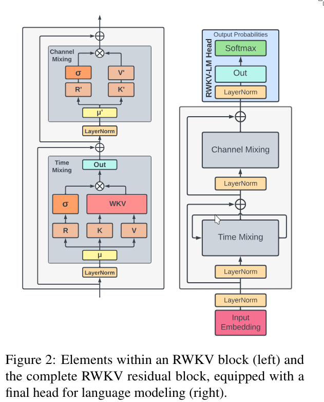
3.3 Architecture
Just like the Transformer architecture is composed of stacked attention blocks, RWKV is made up of multiple RWKV blocks.
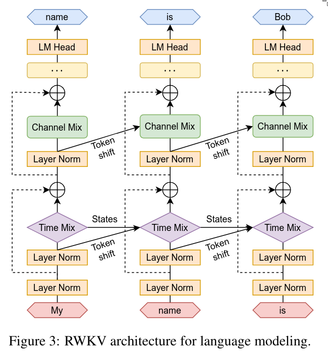
Each RWKV block consists of two main components:
- Time-mixing block
- Channel-mixing block
Additionally, RWKV uses layer normalization to stabilize gradients and residual (skip) connections to improve information flow.
3.4 Token Shift
In self-attention mechanisms, the receptance, key, and value vectors are computed as follows:
$$ r_t = W_r x_t \quad k_t = W_k x_t \quad v_t = W_v x_t $$However, in the RWKV architecture, a technique called token shifting is introduced. This allows each token to access additional information from the token that directly precedes it.
If the network is deep enough, each successive layer can attend to one more previous token. This is analogous to a receptive field in convolutional neural networks: shallow layers see only limited context, while deeper layers have access to a broader one. A similar concept is seen in sliding window attention, where each layer incrementally increases the effective context length. (See: Mistral 7B – Sliding Window Attention).
Token shifting is implemented by interpolating between the current input \(x_t\) and the input from the previous time step \(x_{t-1}\), using a learnable parameter or fixed hyperparameter \(\mu\):
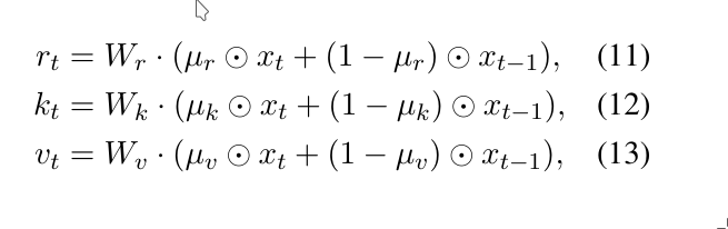
This gives each token some context from the one before it, enabling better temporal understanding without explicit recurrence.
3.5 Channel Mix
In the channel-mixing part of the RWKV block, the previously computed vectors \(r_t\) and \(k_t\) are combined as follows:
$$ o_t = \sigma(r_t) \odot (W_v \cdot \text{ReLU}(k_t)^2) $$Here:
- \(\sigma(r_t)\) is the sigmoid activation, which functions similarly to a forget gate in LSTMs. It controls how much information from the past is allowed to pass through.
- \(\odot\) denotes element-wise multiplication.
- \(\text{ReLU}(k_t)^2\) is the squared ReLU activation function applied to the key vector \(k_t\), serving as a non-linear transformation before being passed through the weight matrix \(W_v\).
This process is very similar to a standard feedforward neural network (FFN), involving:
- Linear transformations via learned weights \(W_r, W_k, W_v\),
- Activation functions,
- And a gating mechanism.
The main differences are:
- The inclusion of token shifting,
- The use of a forget-style gating mechanism \(\sigma(r_t)\).
3.6 Time Mixing
Just like in channel mixing, time mixing also uses the input vectors \(r_t\) and \(k_t\), and additionally includes \(v_t\).
We first compute:
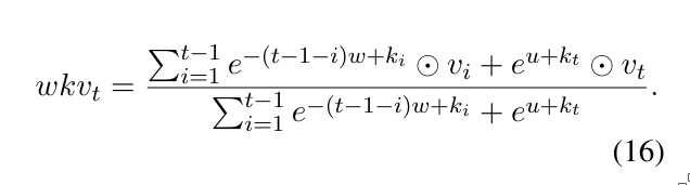
Let’s unpack this. The overall structure follows the pattern of:
$$ \frac{...}{\sum_{i=1}^t e^{-(...)}} \quad \text{(i.e., a softmax function)} $$This structure is used to ensure numerical stability.
Next, consider the part:
$$ \sum_{i=1}^t e^{-(t-1-i)w + k_i} $$Here, we’re summing over all previous time steps (from \(i=1\) to \(t\)). As explained earlier in the motivation section, the term \(-(t - 1 - i)\) computes the distance from the current time step. This is then scaled by a learnable decay vector \(w\). This mechanism ensures that we pay less attention to tokens farther in the past. The result is added to each corresponding key \(k_i\) forming a weighted coefficient for the associated value \(v_i\).
This weighted sum over the past values is then combined with the term \(e^{u + k_t}\), which applies to the current time step. This ensures the current value also influences the final output.
The complete result of this computation is plugged into the following formula:
$$ o_t = W_o \cdot (\sigma(r_t) \odot \text{wkv}_t) $$Here:
- \(\sigma(r_t)\) is a sigmoid gate (similar to an LSTM forget gate),
- \(\odot\) is element-wise multiplication,
- \(\text{wkv}_t\) is the result of the previously discussed weighted sum,
- \(W_o\) is the output weight matrix, applied like a fully connected layer.
3.7 Transformer-like Training
Since both time mixing and channel mixing involve only weighted sums without internal non-linearities, the computations can be rewritten as matrix multiplications. This means we can parallelize the training process, just like in a standard Transformer architecture.
This is possible because the only non-linearities — squared ReLU (in channel mixing) and sigmoid (in time mixing) — are applied after the weighted sum. As a result, the core computation (the sum across past time steps) can be compactly expressed and efficiently computed via matrix operations.
3.8 RNN-like Inference
RWKV offers the best of both worlds:
- Transformer-like parallel training, and
- RNN-like inference with low memory and compute cost.
Since the RWKV block is essentially recursive, inference can be performed step by step, just like in a traditional RNN. This allows efficient deployment, especially in real-time or resource-constrained environments.
Furthermore, unlike Transformers, RWKV’s context length is not fixed. Transformer architectures are constrained by the size of their attention weight matrices, which define a maximum context length. RWKV, on the other hand, can arbitrarily increase context length without changing the model’s size or architecture.
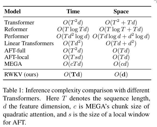
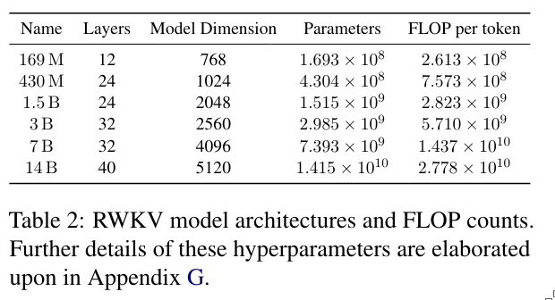
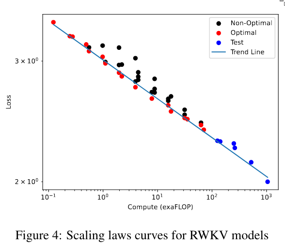
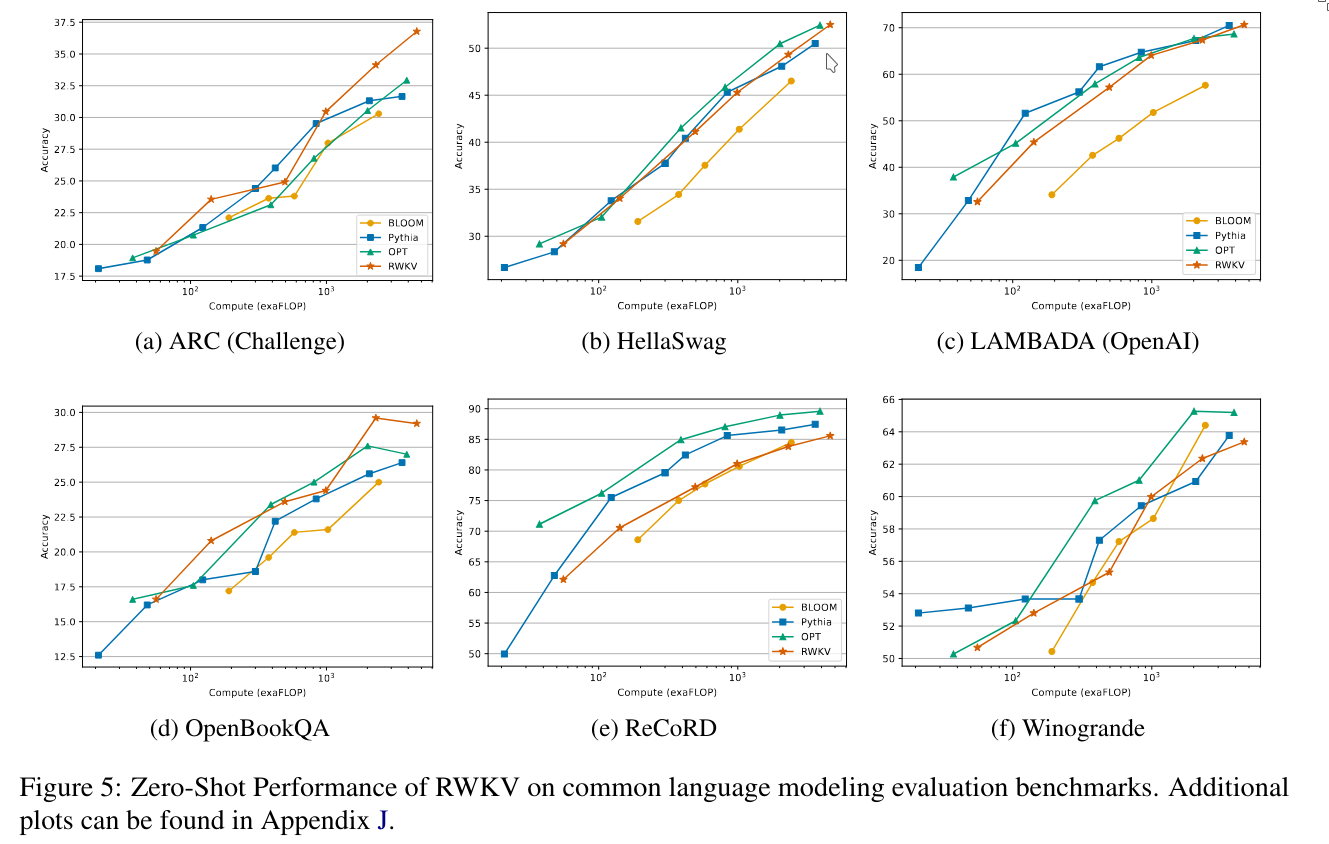
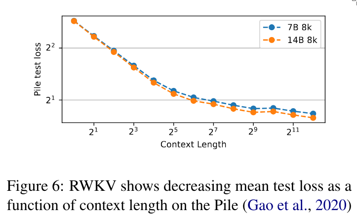
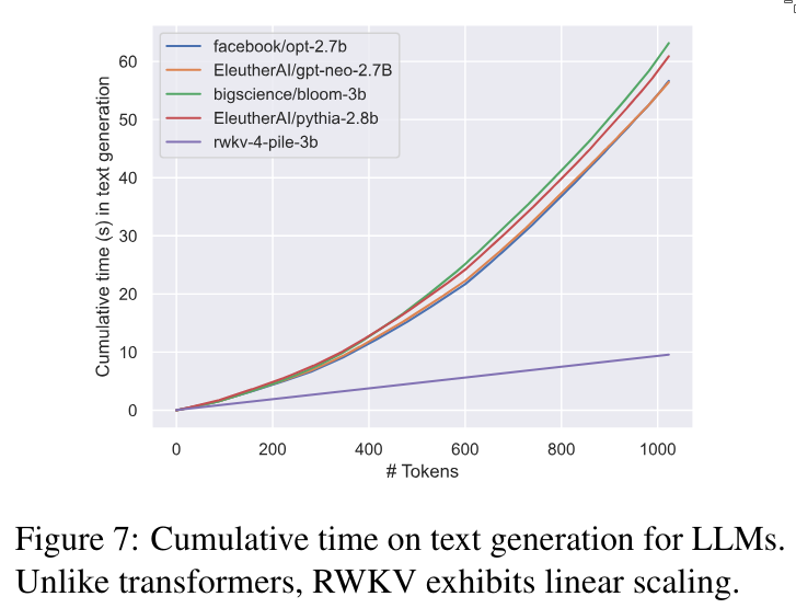
4. Trained model and Computign Costs
Let the graphs speak for themselves.
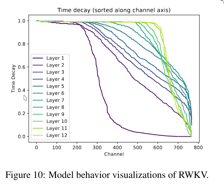
This last figure shows how much attention is paid to different channels at each layer. We can see that in the very early layers, the model focuses on the first channels, while the later channels receive less attention. As we go deeper into the network, the layers begin to focus more on the later channels.
5. Conclusion
RWKV combines the advantages of Transformer training parallelism with the fast inference speed of an RNN. It is also context-independent, meaning the context length can be increased without retraining the model, and it scales similarly to a Transformer.
The main disadvantage of RWKV is that, because it pays less attention to tokens from far back in the sequence, it performs worse on tasks that require remembering details from very long ago.
 reply via email