Spike-based computation using classical recurrent neural networks

October 1, 2025 | 995 words | 5min read

Paper Title: Spike-based computation using classical recurrent neural networks

Link to Paper: https://arxiv.org/abs/2306.03623

Date: 6 May. 2024

Paper Type: Neuromorphic, Architecture, RNN

Short Abstract: This paper introduces a new architecture called the Spiking Recurrent Cell (SRC), inspired by the Gated Recurrent Unit (GRU). This new architecture makes the GRU event-driven through the use of spikes.

1. Introduction

Artificial Neural Networks (ANNs) have become increasingly powerful. However, ANNs require a huge amount of energy for both training and inference. Meanwhile, the brain uses far fewer resources. Inspired by this, Spiking Neural Networks (SNNs) were created, which mimic the spiking neurons in the brain. Such networks need far less energy because of their event-driven nature and can run efficiently on neuromorphic hardware.

There are two major problems with SNNs:

1. Deeper SNNs are often unstable, hard to train, and do not converge.
2. SNNs are not differentiable, and thus cannot be trained using backpropagation. This is often solved by using surrogate gradients.

The authors of this paper aim to solve both issues using their architecture, the Spiking Recurrent Cell (SRC). It is inspired by the GRU, is fully differentiable, and can therefore be trained using backpropagation. Furthermore, it works for deeper neural networks. They modify the architecture to make it event-driven—hence, spiking.

2. Background

2.1 Recurrent Neural Networks

Recurrent Neural Networks (RNNs) are networks with memory, meaning they carry information from their last state, called the hidden state. An RNN is composed of fully connected layers and recurrent neurons. Each recurrent layer has its own hidden state, which is computed from the current input and the previous hidden state. This allows the RNN to model sequences.

Training RNNs is done using backpropagation through time (BPTT). This involves unfolding the RNN in time, effectively making it into a very deep network. As such, BPTT scales with the input sequence length, which is computationally expensive.

RNNs also suffer from the problem of vanishing and exploding gradients. Exploding gradients can be solved with gradient clipping, but often both issues are addressed using gates—mechanisms that control the flow of information (i.e., how much is remembered from previous states and how much is forgotten).

Two of the most famous recurrent cells are the Long Short-Term Memory (LSTM) and the Gated Recurrent Unit (GRU).

2.2 Spiking Neural Networks

In the brain, neurons communicate via spikes—short impulses of electrical signals generated by neuron membranes. There are many models of this phenomenon, but in practice the Leaky Integrate-and-Fire (LIF) model is often used because of its simplicity and computational efficiency.

The LIF works by using a leaky integrator that accumulates input current into a membrane potential. Inputs are added to this potential, which gradually decays over time due to leakage. In addition, there is a reset rule: when the membrane potential reaches a threshold, it resets, and the neuron fires.

Since LIF neurons are non-differentiable, training them is challenging. There are three common solutions:

1. Local plasticity update rules, which do not use backpropagation.
2. Surrogate gradients, where the non-differentiable part of the neuron is replaced with something differentiable during the backward pass.
3. ANN-to-SNN conversion, where a standard ANN is trained and then converted into an SNN.

3. Spiking Recurrent Cell

For the exact mathematical derivation, see the paper.

They started with the formula for a Bistable Recurrent Cell (BRC), which is a variation of the GRU, and then asked how they would need to change it to make it spiking. The idea is that a spike can be described using two steps:

1. a fast local positive feedback that drives the potential to a high value, followed by
2. a slower global negative feedback that brings it back to its resting potential.

This leads to the following model:

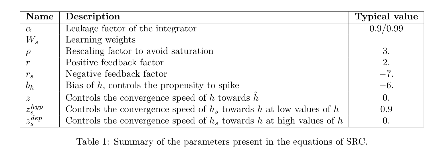
$$ \begin{align} i[t] &= \alpha i[t-1] + W_s s_{in}[t] \tag{5a} \\ x[t] &= \rho \cdot \tanh \left( \frac{i[t]}{\rho} \right) \tag{5b} \\ z_s[h] &= z_s^{hyp} + (z_s^{dep} - z_s^{hyp}) \times H(h[t] - 0.5) \tag{5c} \\ h[t] &= \tanh \left( x[t] + r \odot h[t-1] + r_s \odot h_s[t-1] + b_h \right) \tag{5d} \\ h_s[t] &= z_s[h] \odot h_s[t-1] + (1 - z_s[h]) \odot h[t-1] \tag{5e} \\ s_{out}[t] &= \text{ReLU} \left( h[t] \right) \tag{5f} \end{align} $$

Importantly, only (W) is learnable. The rest of the parameters are set by the authors through experimentation to ensure spiking behavior. This means that during training, the only parameter that changes is (W).

4. Experiments

4.1 Setup

• Implementation: Implemented in PyTorch using the snnTorch library.
• Benchmarks:
  • Datasets: MNIST, Fashion-MNIST, and Neuromorphic-MNIST.
  • Non-neuromorphic datasets were first transformed into spiking data using a firing-rate code.
    • Example: a white pixel spikes with probability 25% (to reduce the number of spikes, not 100%), and a black pixel with probability 0.
• Output: A frozen layer is placed at the end of the network, with one neuron per label.
• Loss Function: Cross-entropy loss.
• Training / Learning:
  • Training is done via backpropagation.
  • During the backward pass, the ReLU derivative is ignored. This improves results, since with standard ReLU the network does not train when there are no output spikes (the derivative would be zero).
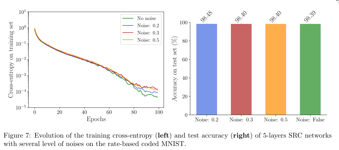
• Ablation:
  • One difference between SRC and LIF is that in LIF, the spike always lasts exactly one timestep. This is not the case for SRC.
  • To check whether the network exploits this property to encode information (which is undesirable), the authors add noise by sampling the parameters (r) and (r_s) from normal distributions.

4.2 Results

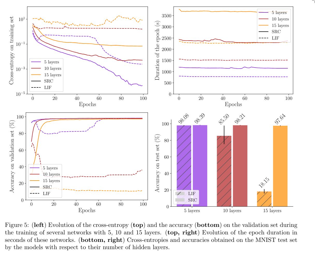
• In shallow networks, SRC achieves comparable or slightly better performance than LIF.

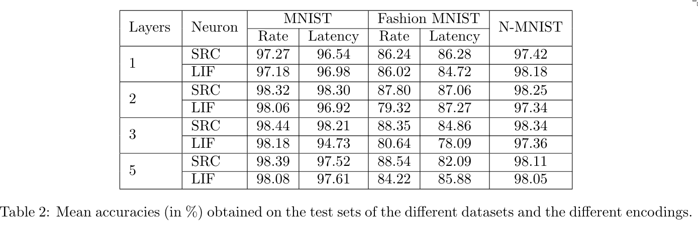
• In deep networks (many layers), SRC vastly outperforms LIF, since LIF fails to learn.

• Adding noise to the parameters does not lead to model collapse. Thus, it can be assumed that SRC networks do not rely on the non-binary shape of their spikes.

5. Results

SRCs combine the advantages of LIF (its spiking nature) with those of modern recurrent architectures like GRU/LSTM, allowing them to work even in deep networks.

---

My Opinions

Too much hand-tuning for my taste. Too many parameters are finely adjusted, which makes the approach feel less generalizable. Remember the bitter lesson.