Training Spiking Neural Network Using Lessongs from Deep Learning
June 24, 2025 | 4,141 words | 20min read
Paper Title: Training Spiking Neural Network Using Lessongs from Deep Learning
Link to Paper: https://arxiv.org/abs/2109.12894
Date: 27. Sep 2021
Paper Type: Neuromorphic-Computing, Spiking Neural Networks, Deep Learning
Short Abstract:
This paper provides an overview of training spiking neural networks (SNNs), which are networks inspired by the brain and use spikes for information propagation. It focuses particularly on how deep learning techniques can be used for SNNs.
This is a very long paper, and I have left out a lot, focusing only on summarizing and writing down what I felt was important.
1. Introduction
Deep learning has solved various problems in diverse fields such as computer vision, speech recognition, and natural language processing.
In particular, large language models (LLMs) like GPT-3 and GPT-4 have recently gained significant prominence for their capabilities. However, these models use billions of parameters. It is estimated that training GPT-3 alone consumed around 190,000 kWh, whereas the human brain only needs around 12–20 watts of power.
If we want to build more efficient models, we should look to the brain for inspiration. One promising direction is neuromorphic computing and spiking neural networks (SNNs).
1.1 Neuromorphic Computing: Characteristics
Neuromorphic (brain-inspired) computing typically involves three components:
Neuromorphic sensors: Inspired by biological systems like the retina. These sensors only generate signals when changes occur; these changes are represented as “spikes.”
Neuromorphic algorithms: These take spike-based input and make sense of it. For example, SNNs use spikes—discrete events instead of floating-point values. Information is encoded over time.
Neuromorphic hardware: Specialized hardware designed to run neuromorphic algorithms as efficiently as possible.
1.2 Neuromorphic Systems in the Wild
The goal of neuromorphic systems is to combine the power of artificial neural networks (ANNs)—like transformers or feedforward networks—with the potential efficiency gains of SNNs.
SNNs have already been successfully deployed in several domains:
- Medicine: For biosignal monitoring (e.g., brain-machine interfaces), where we need to process information locally using low-power devices.
- Robotics: To build more human-like and affordable robots, especially drones that operate in low-power environments.
- Mixed Reality: SNNs can enable more efficient sensory processing.
- Neuroscience: SNNs are also used to study and test theories about how natural intelligence arises and how memory is formed.
2. From Artificial to Spiking Neural Networks
Neural coding refers to how the brain processes and represents information. While the exact mechanisms are still unclear, several theories have emerged:
Spikes: In the brain, neurons communicate through action potentials, or “spikes”—discrete electrical impulses. In computational models, a spike is often represented as a one-bit, all-or-nothing event (i.e., either a spike or no spike). This is more efficient than traditional methods that use floating-point numbers because weights are only multiplied when a spike (“1”) is present.
Sparsity: Sparse tensors—matrices with mostly zeros and few non-zero entries—are efficient to store and compute with. For example:
$$ [0, 0, 0, 0, 1, 0, 0, 0, 0, 1] $$can be represented more efficiently as:
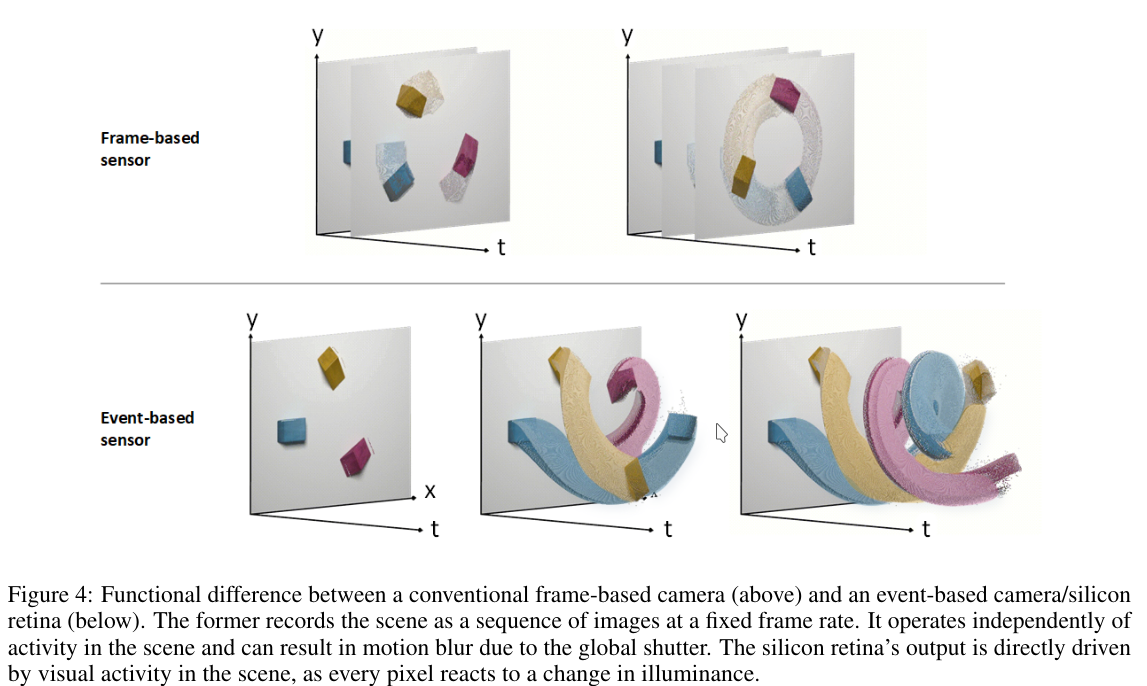
$$ \text{1 at position 5; 1 at position 10} $$Static Suppression (Event-Driven Processing): Sensory systems are more responsive to changes than to static inputs. For example, certain retinal cells react strongly to movement or sudden light changes. A real-life example is the Dynamic Vision Sensor (DVS): unlike a traditional camera that captures every pixel continuously, DVS only records changes in the image.
2.1 Spiking Neuron
ANNs and SNNs can model the same types of network topologies, but the behavior of the individual neuron is different.
Like ANNs, SNNs use weighted sums of inputs \(WX[t]\). However, instead of passing this through an activation function (e.g. sigmoid), the value is added to the membrane potential \(U(t)\). The neuron fires (produces a spike) if the membrane potential reaches a threshold \(\theta\), and then outputs a spike.
The membrane potential \(U(t)\) is time-dependent, since, just like neurons in the brain, SNNs operate continuously rather than in discrete time steps. This is important because we’re not only interested in whether we get a spike or not, but also in how frequently spikes occur—i.e., the spike rate.
Additionally, to prevent the membrane potential from growing infinitely (and to match the behavior of biological neurons), we introduce a decay over time. The parameter \(\beta\) determines the decay rate.
We also need a reset mechanism: when the neuron fires, the membrane potential is reduced by the amount we just fired. This is modeled using the term \(S_{\text{out}}\), which equals 1 when the neuron fires and 0 otherwise.
The full membrane update equation is:
$$ U(t) = \underbrace{\beta U[t -1]}_{\text{decay}} + \underbrace{WX[t]}_{\text{input}} - \underbrace{S_{\text{out}}[t-1] \theta}_{\text{reset}} $$To determine whether a spike occurs, we define:
$$ S_{\text{out}}[t] = \begin{cases} 1, & U[t] > \theta \\ 0, & \text{otherwise} \end{cases} $$This type of neuron is called a Leaky Integrate-and-Fire (LIF) neuron. There are some variations:
- Applying the spike threshold before membrane update.
- Using a hard reset to zero instead of a soft subtraction.
- Scaling the reset term with the decay parameter (e.g., \(\beta S_{\text{out}}[t-1] \theta\)) often improves performance.
Example implementation in Python:
1def lif(X, U):
2    beta = 0.9  # decay rate
3    W = 0.5     # learnable weight
4    theta = 1   # firing threshold
5    S = 0       # output spike
6
7    U = beta * U + W * X - S * theta  # update membrane potential
8    S = int(U > theta)                # determine if a spike occurred
9    return S, U
With snnTorch, this becomes even simpler:
1import snntorch as snn
2
3lif = snn.Leaky(beta=0.9, threshold=1)  # initialize neuron
4
5infinite_loop = True
6while infinite_loop:
7    S, U = lif(X * W, U)  # recurrently update S and U
2.2 Alternative Spiking Neuron Models
There are several other spiking neuron models besides LIF, although they are used less frequently. Some examples include:
- Integrate-and-Fire (IF)
- Current-based models
- Recurrent spiking neurons
- Kernel-based models
- Deep learning–inspired spiking neurons
- High-complexity neuroscience-inspired models
LIF neurons are often preferred for deep learning applications due to their efficiency and similarity to traditional ANN neurons.
If the goal is instead to simulate the brain, more biologically accurate models may be more appropriate.
All of these neuron models can be used in snnTorch.
3. The Neural Code or Data Encodings
The neural code refers to how the brain processes information. For example, light becomes what we “see” when the retina converts photons into spikes. Similarly, odors are perceived when the nose processes molecules into spike patterns.
Broadly, we differentiate between two stages:
- Input encoding — converting input data into spikes that are passed to the network.
- Output encoding — interpreting the output spike patterns of the network.
3.1 Input Encoding
Input data doesn’t necessarily start as spikes—just like the perception of light starts with photons, not spikes.
In fact, static data such as images or audio can be treated as a direct current (DC) input. But this approach doesn’t leverage the full potential of SNNs, which are more meaningful for temporal (i.e., time-varying) data.
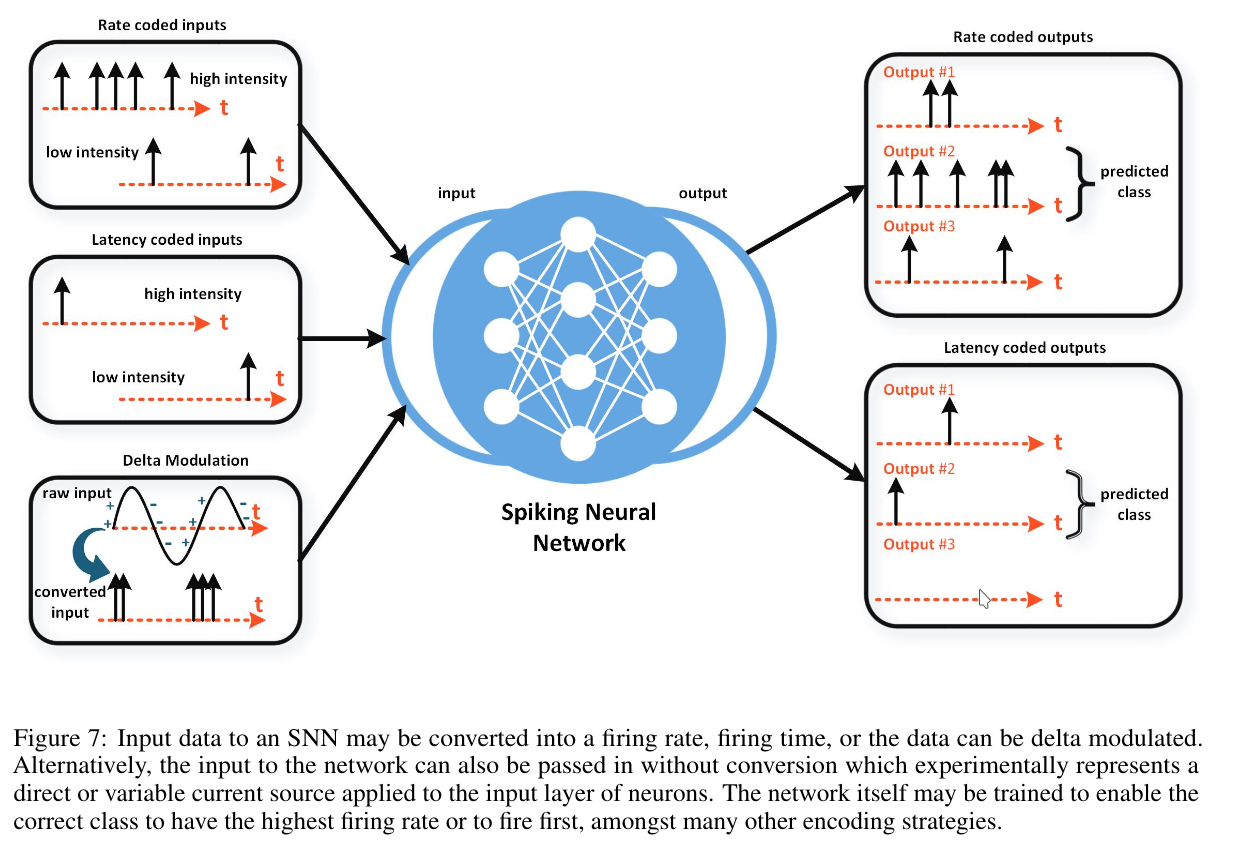
There are three general types of input encodings:
- Rate coding — converts input intensity into firing rate.
- Temporal (or latency) coding — converts input intensity into spike timing.
- Delta modulation — generates spikes only for changes in the input signal, staying silent otherwise.
3.1.1 Rate-Coded Inputs
Our senses convert external stimuli into spike trains. For instance, in vision, brighter light causes neurons to fire more often.
A simple way to implement this is by counting spikes over time. However, this approach loses fine-grained dynamics. A better method uses short time windows, during which the neuron either fires (1) or doesn’t (0). By repeating this process across time steps, we can estimate the likelihood of a spike firing at any given moment. This idea can be extended to multiple neurons, forming a population code.
This method fits well with recurrent models (like RNNs), where each time step acts like one short spike window.
 1from snntorch import spikegen
 2import torch
 3
 4steps = 100  # number of time steps
 5
 6X = torch.rand(10)  # vector of 10 random inputs
 7S = spikegen.rate(X, num_steps=steps)
 8
 9print(X.size())
10# >> torch.Size([10])
11print(S.size())
12# >> torch.Size([100, 10])
3.1.2 Latency-Coded Inputs
In latency (or temporal) coding, the exact timing of a spike carries the information—not how many spikes occur. For instance, a brighter pixel might cause a spike to occur earlier, while a darker one causes a spike to occur later.
This model makes sense biologically: spike processing in the brain is extremely fast, so it’s more likely that the timing of the first spike matters, rather than counting a long sequence of spikes as in rate coding.
 1from snntorch import spikegen
 2import torch
 3
 4steps = 100  # number of time steps
 5
 6X = torch.rand(10)  # vector of 10 random inputs
 7S = spikegen.latency(X, num_steps=steps)
 8
 9print(X.size())
10# >> torch.Size([10])
11print(S.size())
12# >> torch.Size([100, 10])
3.1.3 Delta-Modulated Inputs
The idea of delta modulation is that neurons respond primarily to change rather than to static input. For example, neurons in the retina are less likely to fire if nothing is changing in the visual field.
A common implementation involves defining a threshold: if the difference between inputs exceeds the threshold, a spike is generated.
 1from snntorch import spikegen
 2import torch
 3
 4# Example input tensor: time X batch-size X channel X height X width
 5print(X.size())
 6# >> torch.Size([100, 128, 1, 28, 28])
 7
 8S = spikegen.delta(X, num_steps=steps)  # convert to delta-modulated spikes
 9
10print(S.size())
11# >> torch.Size([100, 128, 1, 28, 28])  # shape remains the same, but values are now spike-encoded
This technique is commonly used to convert normal data into spike format. However, it’s even better to capture data natively as spikes, because you can retain more temporal detail and biological realism.
3.2 Output Decoding
The basic question is: How do we interpret the firing behavior of output neurons?
There are three main decoding strategies:
- Rate Coding: Choose the output neuron with the highest firing rate (i.e., the most spikes over time) as the predicted class.
- Latency Coding: Choose the output neuron that fires first as the predicted class.
- Population Coding: Use a group of neurons per class, and apply rate or latency decoding over that population.
3.2.1 Rate vs. Latency Code
It’s still debated whether the brain predominantly uses rate or latency coding. In practice, each has advantages depending on the task.
Advantages of Rate Coding:
- Error tolerance: If a neuron fails to spike once, others will still spike later.
- Better gradient flow: More spikes provide more learning signals, which often improves performance in training deep networks.
Advantages of Latency Coding:
- Lower power consumption: Fewer spikes mean less energy is used.
- Faster inference: Only the first spike matters, so results can be computed earlier.
Interestingly, biological studies suggest that at most 15% of brain activity can be explained by rate coding. If more used rate coding, our brains would consume far more energy—suggesting that temporal or sparse codes may be more biologically realistic.
3.3 Objective Functions
The brain likely doesn’t use explicit loss functions like cross-entropy. However, processes such as dopamine release are thought to play a role similar to reward signals in reinforcement learning, indirectly shaping neural responses over time.
3.3.1 Spike Rate Objective Functions
There are several types of loss functions that depend on how we want the neurons to behave. Some encourage frequent spiking (rate-based), while others promote precise timing (temporal-based). The choice depends on the application and decoding method.
Here are common loss functions:
- Cross-Entropy Loss:
- Spike Count: Accumulate total spike counts over time.
- Membrane Potential: Use the maximum value of the membrane potential \(U(t)\) during the simulation.
- Mean Square Error (MSE):
- Spike Count: Compare spike counts for all output neurons against target counts.
- Membrane Potential: Define a target potential for each neuron at each time step.
Using spike count is more common, while membrane potential serves as a proxy that works better when you run the model for a limited number of time steps.
Note the differences:
- Cross-entropy suppresses spikes for incorrect classes and can drive irrelevant weights to zero.
- MSE doesn’t suppress firing of incorrect classes, but allows smoother learning when using population codes.
1from snntorch import functional as SF
2
3loss_1 = SF.ce_rate_loss()          # Cross-entropy based on spike count
4loss_2 = SF.mse_rate_loss()         # MSE based on spike count
5loss_3 = SF.ce_max_membrane_loss()  # Cross-entropy based on max membrane potential
6loss_4 = SF.mse_membrane_loss()     # MSE based on membrane potential
3.3.2 Spike Time Objective Functions
Loss functions that rely on spike timing (rather than rate) are less commonly used in deep learning for several reasons:
- Error rate is often the primary concern in machine learning; rate codes are more robust to noise.
- Temporal codes are more biologically accurate, but harder to implement and train due to discrete and sparse spikes.
Still, there are spike-time-specific objective functions, such as:
- Cross-Entropy Spike Time
- Mean Square Spike Time
- Mean Square Relative Spike Time
- Mean Square Membrane
These are used in more biologically inspired models or when spike timing is critical to the task (e.g., fast response systems or event-driven control).
3.4 Learning Rules
3.4.1 Spatial and Temporal Credit Assignment
After defining a loss function, the next step is to update the network to improve its performance on the task. But which weight should be adjusted, and by how much?
This is known as the credit assignment problem—determining how much each weight contributed to the error. It can be split into two sub-problems:
- Spatial credit assignment: Which neuron deserves how much credit (or blame)?
- Temporal credit assignment: At what time should the neuron receive credit?
In traditional deep learning, this is handled by backpropagation. However, it is unlikely that the biological brain performs such an exact algorithm—it would require computing gradients and somehow transmitting them backward through the network, which is biologically implausible.
3.4.2 Biologically Motivated Learning Rules
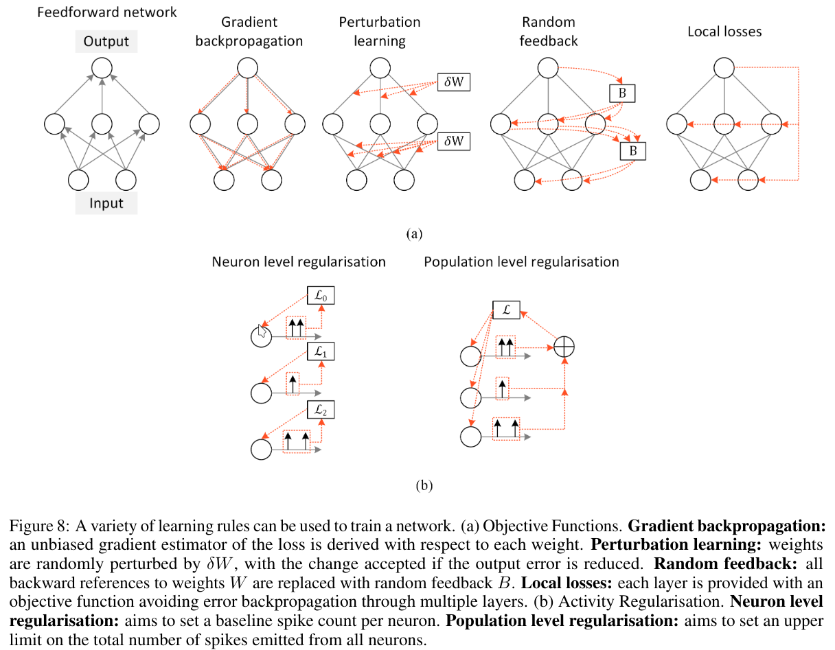
To overcome the biological implausibility of backpropagation, several alternative learning rules have been proposed, inspired by neuroscience:
- Perturbation Learning: Randomly perturbs network weights and observes the change in error. If the error is reduced, the change is accepted; otherwise, it is discarded. This method is simple but requires many trials.
- Random Feedback: Replaces exact feedback weights with random matrices, addressing the weight transport problem (the need to match forward and backward weights).
- Local Losses: Instead of using a global loss function, each layer or module has its own local loss, reducing dependency on global gradient flow.
- Forward-Forward Algorithm: Eliminates the need for a backward pass altogether. Instead, a second forward pass is done where the input signal is perturbed based on error information.
Gradient-based backpropagation is still superior in accuracy and performance, but it’s not always the most efficient or biologically plausible.
Perturbation learning, while conceptually simple, becomes impractical for large models due to the enormous number of trials required.
3.5 Activity Regularisation
One of the main reasons we’re interested in Spiking Neural Networks (SNNs) is their low power consumption. A key factor affecting this is the number of spikes neurons emit—more spikes require more energy.
To manage this, we apply activity regularisation, which penalizes excessive spiking during training. However, there’s a trade-off: too much regularisation can lead to underfiring and poor learning, while too little leads to excessive spiking and higher energy consumption.
We typically distinguish between two types of regularisation:
- Population-Level Regularisation: Controls the total spiking activity across a group of neurons. Useful when optimizing metrics that depend on aggregate behavior.
- Neuron-Level Regularisation: Controls the activity of individual neurons. Important because if a neuron stops firing completely, it may stop contributing to learning.
Experiments show that rate-coded models are generally robust to regularisation, while latency-coded or single-spike models are more sensitive to it.
The key goal is to find a balance—a sweet spot—between too many spikes (wasted energy, noise) and too few spikes (poor learning signal).
4. Training Spiking Neural Networks
There are three general classes of training techniques for SNNs:
Shadow Training: A non-spiking artificial neural network (ANN) is trained using standard methods and later converted into an SNN by interpreting the activations as either firing rates or spike times.
Backpropagation Using Spikes: The SNN is trained directly using error backpropagation, typically through time, as is done with sequential models like RNNs.
Local Learning Rules: Weight updates are computed from signals that are locally available in space and time—unlike backpropagation, which requires a global error signal.
Each method has its own strengths and weaknesses. The focus of this section is on backpropagation.
Backpropagation requires computing the gradient of the loss with respect to the weights. But SNNs involve non-differentiable spike functions. Recall the update equation:
$$ U[t] = \beta U[t-1] + WX[t] $$(Reset terms are omitted for simplicity.)
To compute the gradient \(\Delta W\), we must calculate \(frac{dS}{dU}\), where \(S\) is the spike output. However, since spikes are defined as a hard threshold function, \(\frac{dS}{dU} = 0\) almost everywhere, and \(\frac{dS}{dU} \to \infty\) at the threshold \(\theta\).
This makes the gradient either zero or infinite—neither of which is usable for training.
4.1 Shadow Training
In shadow training, we circumvent this issue entirely by first training a regular ANN using standard deep learning techniques. After training, we convert the ANN into an SNN.
Advantages:
- Allows the use of state-of-the-art training methods, optimizers, and architectures.
- Easier and faster to train due to smooth activations and stable gradients.
Disadvantages:
- No efficiency gains during training (the original reason to use SNNs!).
- Does not utilize temporal dynamics of spiking neurons.
- Conversion can require a large number of simulation time steps.
- The conversion is an approximation, making it hard to recover the original performance.
Hybrid approaches—where training starts with a shadow ANN and then switches to SNN fine-tuning—exist, but they often suffer from accuracy loss post-conversion.
4.2 Backpropagation Using Spike Times
One way to avoid the spike gradient problem is to train using spike timing information. This approach is called SpikeProp.
Instead of relying on the non-differentiable spike function \(S(U)\), it models the firing time as a continuous function \(f(U)\), and computes gradients via \(\frac{df}{dU}\), which is well-defined.
Challenges:
- Neurons that never fire have no gradients; their weights become “frozen.”
- Solutions include careful initialization, but this restricts the use of modern initialization schemes that prevent vanishing/exploding gradients.
- Alternatively, we can lower firing thresholds or use activity regularization, though both tend to hurt performance.
- This approach enforces strong priors: every neuron must fire at least once.
4.3 Backpropagation Using Spikes
The most widely used method is to apply Backpropagation Through Time (BPTT), which is common in training RNNs.
Here’s how it works:
- During the forward pass, the SNN operates normally, including spiking dynamics.
- During the backward pass, gradients are propagated through time, even across time steps where no spikes occurred.
- The total loss is computed as:
- We compute gradients \(\frac{dL}{dW}\) and update weights accordingly.
However, we still face the non-differentiability of the spike function. To address this:
- In the forward pass, we use the true spike function.
- In the backward pass, we replace the derivative \(\frac{dS}{dU}\) with a continuous surrogate, such as the derivative of a sigmoid or piecewise linear function.
This is known as the surrogate gradient method and is currently the most effective way to train SNNs end-to-end with backpropagation.
4.3.1 Surrogate Gradients
Let’s consider a spiking neuron with a threshold \(\theta\). One of the following scenarios applies:
- Membrane potential below threshold: \(U < \theta\) → No spike, derivative is 0
- Membrane potential above threshold: \(U > \theta\) → Spike, but derivative is still 0
- Membrane potential exactly at threshold: \(U = \theta\) Spike, derivative tends to infinity
This discontinuous behavior breaks gradient-based optimization. The solution is to use a surrogate gradient, where we replace the non-differentiable spike function with a smooth approximation during the backward pass. A common choice is a threshold-shifted sigmoid:
$$ \sigma(U) = \frac{1}{1 + e^{\theta - U}} $$This smooth function fixes the issue of infinite or zero gradients in backpropagation.
However, it’s important to note that a spike must still be triggered for a weight update to happen. The surrogate gradient allows gradients to flow backward even from non-spiking neurons, but weight updates still depend on actual spiking activity in the forward pass.
Example in snnTorch:
1import snntorch as snn
2from snntorch import surrogate
3
4lif_1 = snn.Leaky(beta=0.9, spike_grad=surrogate.fast_sigmoid())
5lif_2 = snn.Leaky(beta=0.9, spike_grad=surrogate.sigmoid())
6lif_3 = snn.Leaky(beta=0.9, spike_grad=surrogate.straight_through_estimator())
7lif_4 = snn.Leaky(beta=0.9, spike_grad=surrogate.triangular())
Most state-of-the-art SNN experiments use some form of surrogate gradient for training.
4.3.2 The Link Between Surrogate Gradients and Quantized Neural Networks
In traditional ANNs, Hinton dealt with non-differentiable functions by simply ignoring them during backpropagation, introducing the straight-through estimator (STE). This is equivalent to using a surrogate gradient in SNNs where:
$$ \frac{dS}{dU} = 1 $$This connection links surrogate gradients in SNNs with techniques used in quantized neural networks (QNNs).
Quantization is used to reduce computational cost by using lower-precision number formats:
- Post-training quantization
- Quantization-aware training
- Mixed-precision training
- Binary and ternary neural networks
Interestingly, SNNs are very robust to quantization, especially when trained using quantization-aware methods.
Example:
 1import snntorch as snn
 2import torch.nn as nn
 3import brevitas.nn as qnn
 4
 5# Full-precision model
 6net = nn.Sequential(
 7    nn.Linear(784, 10),
 8    snn.Leaky(beta=0.9, init_hidden=True)
 9)
10
11# Quantized model
12num_bits = 8
13quant_net = nn.Sequential(
14    qnn.QuantLinear(784, 10, weight_bit_width=num_bits),
15    snn.Leaky(beta=0.9, init_hidden=True)
16)
4.3.3 A Bag of Tricks for BPTT in SNNs
Several additional techniques can improve BPTT training of SNNs:
- Ignore the reset mechanism during backpropagation (it’s non-differentiable)
- Residual connections improve gradient flow, just like in deep ANNs
- Learnable decay rates for membrane potential can boost performance
- Graded spikes: scale spike amplitude with a learnable parameter
- Learnable thresholds have not shown significant benefit
- Pooling layers work well for spatial downsampling in SNNs
- Optimizers: Adam is generally effective; for deep SNNs, SGD with momentum can perform better
4.4 Long-Term Temporal Dependencies
Neural time constants in biological brains are typically in the range of 1–100 ms. This makes it difficult for SNNs to handle tasks that require long-term dependencies, such as those found in natural language processing (NLP).
Similar to how LSTMs extended RNNs, SNNs need mechanisms to incorporate longer-range temporal dynamics. Some strategies include:
- Adaptive thresholds: After a neuron fires, it enters a refractory period, making it harder to spike again soon. This creates longer-term memory.
- Recurrent attention mechanisms: Similar to self-attention in transformers, they allow the model to attend to distant time steps or tokens.
- Axonal delays: Introducing artificial propagation delays between neurons can extend the temporal window.
- Membrane dynamics: Modulating decay rate as a function of spike activity can induce second-order effects and richer neuron behavior.
- Multistable neural activity: Also known as attractor networks, these maintain stable activity states over time and are believed to underlie working memory. However, they are very difficult to train effectively.
5. Online Learning
5.1 Temporal Locality
Our brains are remarkable, but it is unlikely that they operate using the Backpropagation Through Time (BPTT) algorithm. Instead, it is far more plausible that biological learning relies on local information available at the present moment.
Therefore, we consider algorithms that adhere to temporal locality, meaning that the gradient depends only on values available at the current time step. One such example is Real-Time Recurrent Learning (RTRL).
5.2 Real-Time Recurrent Learning (RTRL)
RTRL estimates gradients similarly to BPTT but enforces temporal locality. It computes gradients online, step by step, without requiring backward passes over the entire time sequence.
A major advantage is that memory requirements of RTRL do not grow with time \(T\), unlike BPTT, which stores all intermediate states.
However, why isn’t RTRL more widely used in practice? The answer lies in computational complexity: to maintain locality, RTRL needs additional computation rules that result in \(O(n^3)\) memory complexity for a network of size \(n\), while BPTT requires \(O(nT)\). For large networks, \(n^3\) can be prohibitively expensive.
Several variants of RTRL have been proposed to mitigate this, including:
- e-prop (Bellec et al., 2020 [119])
- decolle (Kaiser et al., 2020 [120])
- OSTL (Bohnstingl et al., 2022 [209])
- ETLP (Quintana et al., 2023 [210])
- OSTTP (Ortner and Pes, et al., 2023 [211])
- FPTT (Kag, et al., 2021 [212])
5.3 Spatial Locality
Temporal locality requires the learning rule to depend only on the current state over time. Spatial locality means each weight update depends only on information locally available around that weight — typically the pre- and post-synaptic neurons directly connected by that synapse.
Spatial locality is often considered more biologically plausible.
A classical approach exploiting spatial locality is synaptic plasticity rules, such as Spike-Timing Dependent Plasticity (STDP). In STDP, synaptic weights update based on the precise order and timing of spikes between connected neurons. The underlying idea aligns with the adage:
“Neurons that fire together, wire together.”
It is important to note that backpropagation and STDP do not directly compete:
- Backpropagation is based on global function optimization (gradient descent).
- STDP is a biologically observed, local learning rule describing synaptic changes.
6. Outlook
Spiking neural networks (SNNs) are generally more energy-efficient than traditional artificial neural networks. But the fundamental question remains:
Are spikes actually beneficial for computation?
So far, this question has not been conclusively answered.
 reply via email